marzo 17, 2021
~ 7 MIN
Transformer Encoder
< Blog RSS![]()
Transformer Encoder
En posts anteriores hemos entrado en detalle en los mecanismos de atención utilizados en la arquitectura Transformer. En este post vamos a implementar nuestro primer Transformer completo, en este caso el conocido como Transformer Encoder. Esta arquitectura es utilizada en modelos como BERT o ViT.
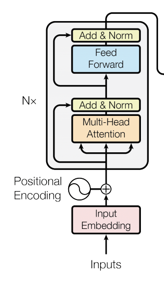
Como puedes ver en la figura, un Transformer no es más que una secuencia de capas formada por:
- El mecanismo de atención multi-head que hemos visto en el post anterior
- Normalización y conexión residual (inspirado en ResNet)
- Un MLP
- Otra normalización y conexión residual
Además, a la entrada de la primera capa, tenemos una etapa de embedding para proyectar nuestros inputs a la dimensión adecuada a la cual añadimos un postitional encoding, el mecanismo que le dirá al transformer en qué posición de la secuencia se encuentra cada vector. Vamos a ver un ejemplo de implementación.
Implementación
import pytorch_lightning as pl
import torch
import matplotlib.pyplot as plt
import torch.nn.functional as F
from sklearn.datasets import fetch_openml
import numpy as np
from torch.utils.data import DataLoader
class Dataset(torch.utils.data.Dataset):
  def __init__(self, X, y):
    self.X = X
    self.y = y

  def __len__(self):
    return len(self.X)

  def __getitem__(self, ix):
    return torch.tensor(self.X[ix]).float(), torch.tensor(self.y[ix]).long()

class MNISTDataModule(pl.LightningDataModule):

    def __init__(self, batch_size: int = 64, Dataset = Dataset):
        super().__init__()
        self.batch_size = batch_size
        self.Dataset = Dataset

    def setup(self, stage=None):
        mnist = fetch_openml('mnist_784', version=1)
        X, y = mnist["data"], mnist["target"]
        X_train, X_test, y_train, y_test = X[:60000] / 255., X[60000:] / 255., y[:60000].astype(np.int), y[60000:].astype(np.int)
        self.train_ds = self.Dataset(X_train, y_train)
        self.val_ds = self.Dataset(X_test, y_test)

    def train_dataloader(self):
        return DataLoader(self.train_ds, batch_size=self.batch_size, shuffle=True)

    def val_dataloader(self):
        return DataLoader(self.val_ds, batch_size=self.batch_size)
dm = MNISTDataModule()
dm.setup()
imgs, labels = next(iter(dm.train_dataloader()))
imgs.shape, labels.shape
(torch.Size([64, 784]), torch.Size([64]))
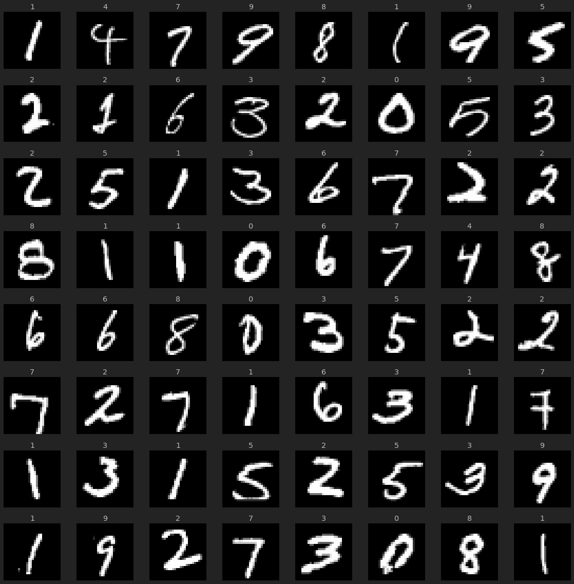
r, c = 8, 8
fig = plt.figure(figsize=(2*c, 2*r))
for _r in range(r):
    for _c in range(c):
        ix = _r*c + _c
        ax = plt.subplot(r, c, ix + 1)
        img, label = imgs[ix], labels[ix]
        ax.axis("off")
        ax.imshow(img.reshape(28,28), cmap="gray")
        ax.set_title(label.item())
plt.tight_layout()
plt.show()
class MLP(pl.LightningModule):

    def __init__(self):
        super().__init__()
        self.mlp = torch.nn.Sequential(
            torch.nn.Linear(784, 784),
            torch.nn.ReLU(inplace=True),
            torch.nn.Linear(784, 10)
        )

    def forward(self, x):
        return self.mlp(x)

    def predict(self, x):
        with torch.no_grad():
          y_hat = self(x)
          return torch.argmax(y_hat, axis=1)

    def compute_loss_and_acc(self, batch):
        x, y = batch
        y_hat = self(x)
        loss = F.cross_entropy(y_hat, y)
        acc = (torch.argmax(y_hat, axis=1) == y).sum().item() / y.shape[0]
        return loss, acc

    def training_step(self, batch, batch_idx):
        loss, acc = self.compute_loss_and_acc(batch)
        self.log('loss', loss)
        self.log('acc', acc, prog_bar=True)
        return loss

    def validation_step(self, batch, batch_idx):
        loss, acc = self.compute_loss_and_acc(batch)
        self.log('val_loss', loss, prog_bar=True)
        self.log('val_acc', acc, prog_bar=True)

    def configure_optimizers(self):
        optimizer = torch.optim.Adam(self.parameters(), lr=0.0003)
        return optimizer
mlp = MLP()
outuput = mlp(torch.randn(64, 784))
outuput.shape
torch.Size([64, 10])
mlp = MLP()
trainer = pl.Trainer(max_epochs=5)
trainer.fit(mlp, dm)
GPU available: True, used: False
TPU available: False, using: 0 TPU cores
/home/sensio/miniconda3/lib/python3.8/site-packages/pytorch_lightning/utilities/distributed.py:45: UserWarning: GPU available but not used. Set the --gpus flag when calling the script.
  warnings.warn(*args, **kwargs)

  | Name | Type       | Params
------------------------------------
0 | mlp  | Sequential | 623 K
/home/sensio/miniconda3/lib/python3.8/site-packages/pytorch_lightning/utilities/distributed.py:45: UserWarning: The dataloader, val dataloader 0, does not have many workers which may be a bottleneck. Consider increasing the value of the `num_workers` argument` (try 20 which is the number of cpus on this machine) in the `DataLoader` init to improve performance.
  warnings.warn(*args, **kwargs)


Validation sanity check: 0it [00:00, ?it/s]


/home/sensio/miniconda3/lib/python3.8/site-packages/pytorch_lightning/utilities/distributed.py:45: UserWarning: The dataloader, train dataloader, does not have many workers which may be a bottleneck. Consider increasing the value of the `num_workers` argument` (try 20 which is the number of cpus on this machine) in the `DataLoader` init to improve performance.
  warnings.warn(*args, **kwargs)


Training: 0it [00:00, ?it/s]


Validating: 0it [00:00, ?it/s]


Validating: 0it [00:00, ?it/s]


Validating: 0it [00:00, ?it/s]


Validating: 0it [00:00, ?it/s]


Validating: 0it [00:00, ?it/s]


1
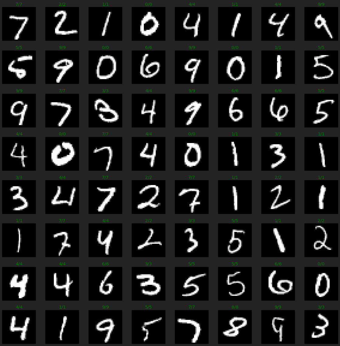
Obtenemos una precisión en los datos de validación del 97%, nada impresionante debido a la simplicidad del modelo.
imgs, labels = next(iter(dm.val_dataloader()))
preds = mlp.predict(imgs)

r, c = 8, 8
fig = plt.figure(figsize=(2*c, 2*r))
for _r in range(r):
    for _c in range(c):
        ix = _r*c + _c
        ax = plt.subplot(r, c, ix + 1)
        img, label = imgs[ix], labels[ix]
        ax.axis("off")
        ax.imshow(img.reshape(28,28), cmap="gray")
        ax.set_title(f'{label.item()}/{preds[ix].item()}', color="green" if label == preds[ix] else 'red')
plt.tight_layout()
plt.show()
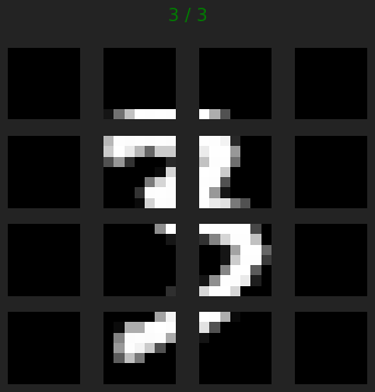
Vamos ahora a resolver el mismo problema, utilizando un Transformer. Lo primero que tenemos que tener en cuenta es que los mecanismos de atención funcionan con secuencias, por lo que tenemos que reinterpretar nuestras imágenes. Para ello, vamos a dividirlas en 16 patches de 7x7. De esta manera, nuestras imágenes ahora serán secuencias de patches con las que nuestro mecanismo de atención podrá trabajar.
class AttnDataset(torch.utils.data.Dataset):
  def __init__(self, X, y, patch_size=(7, 7)):
    self.X = X
    self.y = y
    self.patch_size = patch_size

  def __len__(self):
    return len(self.X)

  def __getitem__(self, ix):
    image = torch.tensor(self.X[ix]).float().view(28, 28) # 28 x 28
    h, w = self.patch_size
    patches = image.unfold(0, h, h).unfold(1, w, w) # 4 x 4 x 7 x 7
    patches = patches.contiguous().view(-1, h*w) # 16 x 49
    return patches, torch.tensor(self.y[ix]).long()
attn_dm = MNISTDataModule(Dataset = AttnDataset)
attn_dm.setup()
imgs, labels = next(iter(attn_dm.train_dataloader()))
imgs.shape, labels.shape
(torch.Size([64, 16, 49]), torch.Size([64]))
import matplotlib
import matplotlib.pyplot as plt
import matplotlib.gridspec as gridspec

fig = plt.figure(figsize=(5,5))
for i in range(4):
    for j in range(4):
        ax = plt.subplot(4, 4, i*4 + j + 1)
        ax.imshow(imgs[6,i*4 + j].view(7, 7), cmap="gray")
        ax.axis('off')
plt.tight_layout()
plt.show()

# basado en: https://github.com/karpathy/minGPT/blob/master/mingpt/model.py
import math

class MultiHeadAttention(torch.nn.Module):

    def __init__(self, n_embd, n_heads):
        super().__init__()
        self.n_heads = n_heads

        # key, query, value projections
        self.key = torch.nn.Linear(n_embd, n_embd*n_heads)
        self.query = torch.nn.Linear(n_embd, n_embd*n_heads)
        self.value = torch.nn.Linear(n_embd, n_embd*n_heads)

        # output projection
        self.proj = torch.nn.Linear(n_embd*n_heads, n_embd)

    def forward(self, x):
        B, L, F = x.size()

        # calculate query, key, values for all heads in batch and move head forward to be the batch dim
        k = self.key(x).view(B, L, F, self.n_heads).transpose(1, 3) # (B, nh, L, F)
        q = self.query(x).view(B, L, F, self.n_heads).transpose(1, 3) # (B, nh, L, F)
        v = self.value(x).view(B, L, F, self.n_heads).transpose(1, 3) # (B, nh, L, F)

        # attention (B, nh, L, F) x (B, nh, F, L) -> (B, nh, L, L)
        att = (q @ k.transpose(-2, -1)) * (1.0 / math.sqrt(k.size(-1)))
        att = torch.nn.functional.softmax(att, dim=-1)
        y = att @ v # (B, nh, L, L) x (B, nh, L, F) -> (B, nh, L, F)
        y = y.transpose(1, 2).contiguous().view(B, L, F*self.n_heads) # re-assemble all head outputs side by side

        return self.proj(y)

class TransformerBlock(torch.nn.Module):
    def __init__(self, n_embd, n_heads):
        super().__init__()
        self.ln1 = torch.nn.LayerNorm(n_embd)
        self.ln2 = torch.nn.LayerNorm(n_embd)
        self.attn = MultiHeadAttention(n_embd, n_heads)
        self.mlp = torch.nn.Sequential(
            torch.nn.Linear(n_embd, 4 * n_embd),
            torch.nn.ReLU(),
            torch.nn.Linear(4 * n_embd, n_embd),
        )

    def forward(self, x):
        x = self.ln1(x + self.attn(x))
        x = self.ln2(x + self.mlp(x))
        return x

class Model(MLP):

    def __init__(self, n_input=7*7, n_embd=7*7, seq_len=4*4, n_heads=4*4, n_layers=1):
        super().__init__()
        self.mlp = None
        self.pos_emb = torch.nn.Parameter(torch.zeros(1, seq_len, n_embd))
        self.inp_emb = torch.nn.Linear(n_input, n_embd)
        self.tranformer = torch.nn.Sequential(*[TransformerBlock(n_embd, n_heads) for _ in range(n_layers)])
        self.fc = torch.nn.Linear(n_embd*seq_len, 10)

    def forward(self, x):
        # embedding
        e = self.inp_emb(x) + self.pos_emb
        # transformer blocks
        x = self.tranformer(e)
        # classifier
        y = self.fc(x.view(x.size(0), -1))
        return y
model = Model(n_layers=3)
trainer = pl.Trainer(max_epochs=5, gpus=1)
trainer.fit(model, attn_dm)
GPU available: True, used: True
TPU available: False, using: 0 TPU cores
LOCAL_RANK: 0 - CUDA_VISIBLE_DEVICES: [0]

  | Name       | Type       | Params
------------------------------------------
0 | inp_emb    | Linear     | 2 K
1 | tranformer | Sequential | 527 K
2 | fc         | Linear     | 7 K


Validation sanity check: 0it [00:00, ?it/s]


Training: 0it [00:00, ?it/s]


Validating: 0it [00:00, ?it/s]


Validating: 0it [00:00, ?it/s]


Validating: 0it [00:00, ?it/s]


Validating: 0it [00:00, ?it/s]


Validating: 0it [00:00, ?it/s]


1
Nuestro Transformer es capaz de clasificar mejor las imágenes con un número similar (ligeramente inferior) de parámetros.
import random

attn_imgs, attn_labels = next(iter(attn_dm.val_dataloader()))
preds = model.predict(attn_imgs)

ix = random.randint(0,attn_dm.batch_size)
fig = plt.figure(figsize=(5,5))
for i in range(4):
    for j in range(4):
        ax = plt.subplot(4, 4, i*4 + j + 1)
        ax.imshow(attn_imgs[ix,i*4 + j].view(7, 7), cmap="gray")
        ax.axis('off')
fig.suptitle(f'{attn_labels[ix]} / {preds[ix].item()}', color="green" if attn_labels[ix] == preds[ix].item() else "red")
plt.tight_layout()
plt.show()
Resumen
En este post hemos implementado nuestro primer Transformer 🎊 Para ello hemos usado el mecanismo de atención desarrollado en los posts anteriores y añadido el resto de piezas incluídas en el artículo original: Capas de normalización, conexiones residuales y un MLP. Además, hemos aprendido a proyectar nuestros inputs a la dimensión necesaria y permitirle al modelo a conocer la posición de cada vector en la secuencia. usando embeddings