julio 7, 2021
~ 14 MIN
Pytorch Profiler
< Blog RSS![]()
Pytorch - Profiling
En posts anteriores hemos visto mucho ejemplos de lo que podemos llegar a hacer con Pytorch, nuestra librería favorita (al menos de momento 😛) para implementar y entrenar redes neuronales. Sin embargo nunca nos hemos preocupado por cómo de óptimo era nuestro código. En este post y los que vienen a continuación nos vamos a enfocar precisamente de ello.
Para empezar, vamos a reutilizar el código para entrenar una red convolucional en el dataset CIFAR10 que ya hemos usado en posts anteriores. Primero definimos nuestro Dataset, que se encargará de leer las imágenes.
import torch
import torchvision
import numpy as np

class Dataset(torch.utils.data.Dataset):
    def __init__(self, train=True):
        trainset = torchvision.datasets.CIFAR10(root='./data', train=train, download=True)
        self.classes = ('plane', 'car', 'bird', 'cat', 'deer', 'dog', 'frog', 'horse', 'ship', 'truck')
        self.imgs, self.labels = np.array([np.array(i[0]) for i in trainset]), np.array([i[1] for i in trainset])
    def __len__(self):
        return len(self.imgs)
    def __getitem__(self, ix):
        img = self.imgs[ix]
        return torch.from_numpy(img / 255.).permute(2,0,1).float(), torch.tensor(self.labels[ix]).long()

ds = {
    'train': Dataset(),
    'test': Dataset(train=False)
}
Downloading https://www.cs.toronto.edu/~kriz/cifar-10-python.tar.gz to ./data/cifar-10-python.tar.gz


HBox(children=(HTML(value=''), FloatProgress(value=0.0, max=170498071.0), HTML(value='')))


Extracting ./data/cifar-10-python.tar.gz to ./data
Files already downloaded and verified
A continuación definimos el DataLoader, que se encargará de alimentar la red neuronal con batches de imágenes.
batch_size = 32

dl = {
    'train': torch.utils.data.DataLoader(ds['train'], batch_size=batch_size, shuffle=True),
    'test': torch.utils.data.DataLoader(ds['test'], batch_size=batch_size, shuffle=False)
}
imgs, labels = next(iter(dl['train']))
imgs.shape, labels.shape
(torch.Size([32, 3, 32, 32]), torch.Size([32]))
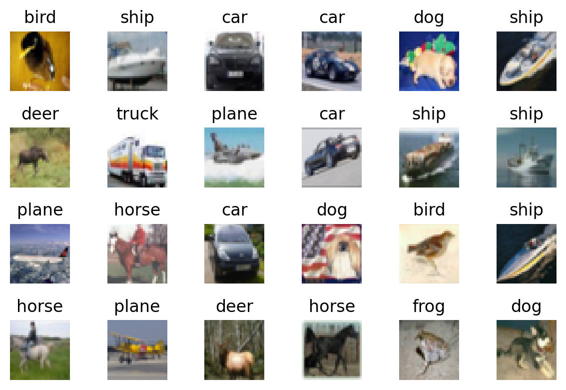
import matplotlib.pyplot as plt

fig = plt.figure(dpi=200)
c, r = 6, 4
for j in range(r):
    for i in range(c):
        ix = j*c + i
        ax = plt.subplot(r, c, ix + 1)
        img, label = imgs[ix], labels[ix]
        ax.imshow(img.permute(1,2,0))
        ax.set_title(ds['train'].classes[label.item()])
        ax.axis('off')
plt.tight_layout()
plt.show()
Usaremos una resnet18 pre-entranada a la cual cambiaremos la última capa para poder llevar a cabo la tarea de clasificación en 10 clases.
import torch.nn.functional as F

class Model(torch.nn.Module):

    def __init__(self, n_outputs=10):
        super().__init__()
        self.model = torchvision.models.resnet18(pretrained=True)
        self.model.fc = torch.nn.Linear(512, n_outputs)

    def forward(self, x):
        return self.model(x)
model = Model()
output = model(torch.randn(32, 3, 32, 32))

output.shape
torch.Size([32, 10])
A continuación definimos nuestras funciones de entrenamiento.
from tqdm import tqdm

def step(model, batch, device):
    x, y = batch
    x, y = x.to(device), y.to(device)
    y_hat = model(x)
    loss = F.cross_entropy(y_hat, y)
    acc = (torch.argmax(y_hat, axis=1) == y).sum().item() / y.size(0)
    return loss, acc

def train(model, dl, optimizer, epochs=10, device="cpu", prof=None, end=0):
    model.to(device)
    hist = {'loss': [], 'acc': [], 'test_loss': [], 'test_acc': []}
    for e in range(1, epochs+1):
        # train
        model.train()
        l, a = [], []
        bar = tqdm(dl['train'])
        stop=False
        for batch_idx, batch in enumerate(bar):
            optimizer.zero_grad()
            loss, acc = step(model, batch, device)
            loss.backward()
            optimizer.step()
            l.append(loss.item())
            a.append(acc)
            bar.set_description(f"training... loss {np.mean(l):.4f} acc {np.mean(a):.4f}")
            # profiling
            if prof:
                if batch_idx >= end:
                    stop = True
                    break
                prof.step()
        hist['loss'].append(np.mean(l))
        hist['acc'].append(np.mean(a))
        if stop:
            break
        # eval
        model.eval()
        l, a = [], []
        bar = tqdm(dl['test'])
        with torch.no_grad():
            for batch in bar:
                loss, acc = step(model, batch, device)
                l.append(loss.item())
                a.append(acc)
                bar.set_description(f"testing... loss {np.mean(l):.4f} acc {np.mean(a):.4f}")
        hist['test_loss'].append(np.mean(l))
        hist['test_acc'].append(np.mean(a))
        # log
        log = f'Epoch {e}/{epochs}'
        for k, v in hist.items():
            log += f' {k} {v[-1]:.4f}'
        print(log)

    return hist
Finalmente, podemos entrenar nuestro modelo.
model = Model()
optimizer = torch.optim.Adam(model.parameters(), lr=1e-3)

hist = train(model, dl, optimizer, epochs=3)
training... loss 1.0930 acc 0.6304: 100%|██████████| 1563/1563 [01:18<00:00, 19.92it/s]
testing... loss 0.9886 acc 0.6755: 100%|██████████| 313/313 [00:03<00:00, 95.14it/s]
training... loss 0.8019 acc 0.7188:   0%|          | 3/1563 [00:00<01:16, 20.31it/s]

Epoch 1/3 loss 1.0930 acc 0.6304 test_loss 0.9886 test_acc 0.6755


training... loss 0.7577 acc 0.7452: 100%|██████████| 1563/1563 [01:18<00:00, 19.81it/s]
testing... loss 0.7643 acc 0.7420: 100%|██████████| 313/313 [00:03<00:00, 99.71it/s]
training... loss 0.5882 acc 0.8281:   0%|          | 3/1563 [00:00<01:16, 20.28it/s]

Epoch 2/3 loss 0.7577 acc 0.7452 test_loss 0.7643 test_acc 0.7420


training... loss 0.6391 acc 0.7842: 100%|██████████| 1563/1563 [01:18<00:00, 19.97it/s]
testing... loss 0.7600 acc 0.7496: 100%|██████████| 313/313 [00:03<00:00, 91.55it/s]

Epoch 3/3 loss 0.6391 acc 0.7842 test_loss 0.7600 test_acc 0.7496
Si bien hemos conseguido nuestro objetivo de entrenar esta red neuronal, ¿acaso lo hemos hecho de la manera más óptima? O dicho de otra manera, ¿sería posible utilizar el hardware que tenemos a nuestra disposición para poder entrenar nuestro modelo más rápido? Para poder responder a estas preguntas necesitamos alguna manera de trackear todas las operaciones que tienen lugar durante el entrenamiento y guardar el tiempo o memoria utilizado por cada una de ellas. Para ello podemos usar una herramienta conocida como Profiler.
El Profiler
Lo primero que podemos medir es el tiempo que nuestro modelo invierte en cada una de las operaciones involucradas.
El
profilerfue introducido en la versión 1.8.1 dePytorch, así que aségurate de tener una versión compatible !
from torch.profiler import profile, record_function, ProfilerActivity

torch.__version__
'1.8.1'
with profile(activities=[ProfilerActivity.CPU], record_shapes=True) as prof:
    with record_function("model_inference"):
        model(torch.randn(32, 3, 32, 32))
print(prof.key_averages().table(sort_by="cpu_time_total", row_limit=20))
---------------------------------  ------------  ------------  ------------  ------------  ------------  ------------
                             Name    Self CPU %      Self CPU   CPU total %     CPU total  CPU time avg    # of Calls
---------------------------------  ------------  ------------  ------------  ------------  ------------  ------------
                  model_inference        10.91%       2.392ms        99.72%      21.856ms      21.856ms             1
                     aten::conv2d         0.68%     149.000us        56.77%      12.442ms     622.100us            20
                aten::convolution         0.67%     146.000us        56.09%      12.293ms     614.650us            20
               aten::_convolution         1.13%     247.000us        55.42%      12.147ms     607.350us            20
         aten::mkldnn_convolution        53.72%      11.774ms        54.30%      11.900ms     595.000us            20
                 aten::batch_norm         0.54%     118.000us        15.49%       3.394ms     169.700us            20
     aten::_batch_norm_impl_index         0.86%     189.000us        14.95%       3.276ms     163.800us            20
          aten::native_batch_norm        12.27%       2.689ms        13.95%       3.058ms     152.900us            20
                 aten::max_pool2d         0.04%       9.000us         7.10%       1.557ms       1.557ms             1
    aten::max_pool2d_with_indices         7.00%       1.534ms         7.06%       1.548ms       1.548ms             1
                      aten::randn         0.10%      22.000us         3.37%     738.000us     738.000us             1
                      aten::relu_         1.03%     226.000us         3.21%     704.000us      41.412us            17
                    aten::normal_         3.06%     670.000us         3.06%     670.000us     670.000us             1
                 aten::threshold_         2.18%     478.000us         2.18%     478.000us      28.118us            17
                       aten::add_         1.85%     405.000us         1.85%     405.000us      50.625us             8
                 aten::empty_like         1.17%     257.000us         1.68%     369.000us       6.150us            60
                      aten::empty         1.38%     302.000us         1.38%     302.000us       2.822us           107
        aten::adaptive_avg_pool2d         0.03%       7.000us         0.47%     104.000us     104.000us             1
                     aten::linear         0.05%      11.000us         0.46%     100.000us     100.000us             1
                       aten::mean         0.07%      15.000us         0.44%      97.000us      97.000us             1
---------------------------------  ------------  ------------  ------------  ------------  ------------  ------------
Self CPU time total: 21.917ms
Podemos ver que nuestro modelo se pasa la mayor parte del tiempo calculando convoluciones, y después batch norm. Algo importante a remarcar es la diferencia en Self CPU y CPU total. En el primer caso se calcula el tiempo invertido en el operador, pero no en llamadas a otros operadores, lo cual sí ocurre en el segundo caso.
Podemos agrupar los operadores por tamaños de tensores para obtener más información.
print(prof.key_averages(group_by_input_shape=True).table(sort_by="cpu_time_total", row_limit=10))
---------------------------------  ------------  ------------  ------------  ------------  ------------  ------------  ---------------------------------------------
                             Name    Self CPU %      Self CPU   CPU total %     CPU total  CPU time avg    # of Calls                                   Input Shapes
---------------------------------  ------------  ------------  ------------  ------------  ------------  ------------  ---------------------------------------------
                  model_inference        10.91%       2.392ms        99.72%      21.856ms      21.856ms             1                                             []
                     aten::conv2d         0.12%      26.000us        14.27%       3.128ms     782.000us             4  [[32, 64, 8, 8], [64, 64, 3, 3], [], [], [],
                aten::convolution         0.15%      32.000us        14.15%       3.102ms     775.500us             4  [[32, 64, 8, 8], [64, 64, 3, 3], [], [], [],
               aten::_convolution         0.25%      55.000us        14.01%       3.070ms     767.500us             4  [[32, 64, 8, 8], [64, 64, 3, 3], [], [], [],
                     aten::conv2d         0.10%      21.000us        13.86%       3.038ms       1.013ms             3  [[32, 512, 1, 1], [512, 512, 3, 3], [], [], [
                aten::convolution         0.08%      18.000us        13.77%       3.017ms       1.006ms             3  [[32, 512, 1, 1], [512, 512, 3, 3], [], [], [
         aten::mkldnn_convolution        13.65%       2.992ms        13.76%       3.015ms     753.750us             4  [[32, 64, 8, 8], [64, 64, 3, 3], [], [], [],
               aten::_convolution         0.15%      33.000us        13.68%       2.999ms     999.667us             3  [[32, 512, 1, 1], [512, 512, 3, 3], [], [], [
         aten::mkldnn_convolution        13.44%       2.945ms        13.53%       2.966ms     988.667us             3  [[32, 512, 1, 1], [512, 512, 3, 3], [], [], [
                     aten::conv2d         0.09%      19.000us         7.22%       1.582ms     527.333us             3  [[32, 256, 2, 2], [256, 256, 3, 3], [], [], [
---------------------------------  ------------  ------------  ------------  ------------  ------------  ------------  ---------------------------------------------
Self CPU time total: 21.917ms
Y también visualizar la cantidad de memoria utilizada por el modelo.
with profile(activities=[ProfilerActivity.CPU], profile_memory=True, record_shapes=True) as prof:
    model(torch.randn(32, 3, 32, 32))

print(prof.key_averages().table(sort_by="self_cpu_memory_usage", row_limit=10))
---------------------------------  ------------  ------------  ------------  ------------  ------------  ------------  ------------  ------------
                             Name    Self CPU %      Self CPU   CPU total %     CPU total  CPU time avg       CPU Mem  Self CPU Mem    # of Calls
---------------------------------  ------------  ------------  ------------  ------------  ------------  ------------  ------------  ------------
                      aten::empty         1.46%     490.000us         1.46%     490.000us       4.667us      12.85 Mb      12.85 Mb           105
                    aten::resize_         0.03%      11.000us         0.03%      11.000us       5.500us       1.50 Mb       1.50 Mb             2
                      aten::addmm         0.22%      74.000us         0.26%      88.000us      88.000us       1.25 Kb       1.25 Kb             1
                        aten::add         0.97%     324.000us         0.97%     324.000us      16.200us         160 b         160 b            20
              aten::empty_strided         0.01%       4.000us         0.01%       4.000us       4.000us           4 b           4 b             1
                      aten::randn         0.11%      38.000us         4.58%       1.538ms       1.538ms     384.00 Kb           0 b             1
                    aten::normal_         4.19%       1.404ms         4.19%       1.404ms       1.404ms           0 b           0 b             1
                     aten::conv2d         0.51%     172.000us        36.29%      12.175ms     608.750us       6.19 Mb           0 b            20
                aten::convolution         0.83%     279.000us        35.78%      12.003ms     600.150us       6.19 Mb           0 b            20
               aten::_convolution         0.86%     288.000us        34.95%      11.724ms     586.200us       6.19 Mb           0 b            20
---------------------------------  ------------  ------------  ------------  ------------  ------------  ------------  ------------  ------------
Self CPU time total: 33.548ms
Mejora 1 - Ejección en GPU
Si estas familiarizado con el entrenamiento de redes neuronales, o has seguido un poco la actividad en este blog, no te sorprenderá que la primera mejora que podemos hacer a nuestro código es la de entrenar el modelo en la GPU.
model = Model()
optimizer = torch.optim.Adam(model.parameters(), lr=1e-3)

hist = train(model, dl, optimizer, epochs=3, device="cuda")
training... loss 1.1143 acc 0.6274: 100%|██████████| 1563/1563 [00:21<00:00, 71.33it/s]
testing... loss 1.0616 acc 0.6560: 100%|██████████| 313/313 [00:01<00:00, 231.94it/s]
training... loss 0.9434 acc 0.6897:   1%|          | 8/1563 [00:00<00:21, 71.66it/s]

Epoch 1/3 loss 1.1143 acc 0.6274 test_loss 1.0616 test_acc 0.6560


training... loss 0.7789 acc 0.7404: 100%|██████████| 1563/1563 [00:21<00:00, 73.30it/s]
testing... loss 0.8353 acc 0.7164: 100%|██████████| 313/313 [00:01<00:00, 223.07it/s]
training... loss 0.6705 acc 0.7790:   1%|          | 8/1563 [00:00<00:21, 71.25it/s]

Epoch 2/3 loss 0.7789 acc 0.7404 test_loss 0.8353 test_acc 0.7164


training... loss 0.6476 acc 0.7855: 100%|██████████| 1563/1563 [00:21<00:00, 73.31it/s]
testing... loss 0.7857 acc 0.7637: 100%|██████████| 313/313 [00:01<00:00, 239.56it/s]

Epoch 3/3 loss 0.6476 acc 0.7855 test_loss 0.7857 test_acc 0.7637
Podemos ejecutar el profiler también en la GPU de la siguiente manera.
with profile(activities=[ProfilerActivity.CPU, ProfilerActivity.CUDA], profile_memory=True, record_shapes=True) as prof:
    with record_function("model_inference"):
        model(torch.randn(32, 3, 32, 32).cuda())

print(prof.key_averages().table(sort_by="cuda_time_total", row_limit=10))
-------------------------------------------------------  ------------  ------------  ------------  ------------  ------------  ------------  ------------  ------------  ------------  ------------  ------------  ------------  ------------  ------------
                                                   Name    Self CPU %      Self CPU   CPU total %     CPU total  CPU time avg     Self CUDA   Self CUDA %    CUDA total  CUDA time avg       CPU Mem  Self CPU Mem      CUDA Mem  Self CUDA Mem    # of Calls
-------------------------------------------------------  ------------  ------------  ------------  ------------  ------------  ------------  ------------  ------------  ------------  ------------  ------------  ------------  ------------  ------------
                                        model_inference         0.12%       1.437ms       100.00%        1.160s        1.160s       0.000us         0.00%       1.782ms       1.782ms          -4 b    -384.02 Kb           0 b     -14.31 Mb             1
                                           aten::conv2d         0.01%     122.000us        99.37%        1.153s      57.646ms       0.000us         0.00%       1.570ms      78.500us           0 b           0 b       6.19 Mb           0 b            20
                                      aten::convolution         0.01%     106.000us        99.36%        1.153s      57.640ms       0.000us         0.00%       1.570ms      78.500us           0 b           0 b       6.19 Mb           0 b            20
                                     aten::_convolution         0.01%     171.000us        99.35%        1.153s      57.634ms       0.000us         0.00%       1.570ms      78.500us           0 b           0 b       6.19 Mb           0 b            20
                                aten::cudnn_convolution         0.13%       1.466ms        99.34%        1.153s      57.626ms       1.570ms        88.10%       1.570ms      78.500us           0 b           0 b       6.19 Mb    -141.64 Mb            20
                                ampere_sgemm_128x128_nn         0.00%       0.000us         0.00%       0.000us       0.000us     387.000us        21.72%     387.000us     129.000us           0 b           0 b           0 b           0 b             3
void implicit_convolve_sgemm<float, float, 128, 6, 7...         0.00%       0.000us         0.00%       0.000us       0.000us     298.000us        16.72%     298.000us     149.000us           0 b           0 b           0 b           0 b             2
void implicit_convolve_sgemm<float, float, 128, 5, 5...         0.00%       0.000us         0.00%       0.000us       0.000us     228.000us        12.79%     228.000us      45.600us           0 b           0 b           0 b           0 b             5
ampere_scudnn_winograd_128x128_ldg1_ldg4_relu_tile44...         0.00%       0.000us         0.00%       0.000us       0.000us     222.000us        12.46%     222.000us      37.000us           0 b           0 b           0 b           0 b             6
void cudnn::winograd_nonfused::winogradForwardFilter...         0.00%       0.000us         0.00%       0.000us       0.000us     171.000us         9.60%     171.000us      57.000us           0 b           0 b           0 b           0 b             3
-------------------------------------------------------  ------------  ------------  ------------  ------------  ------------  ------------  ------------  ------------  ------------  ------------  ------------  ------------  ------------  ------------
Self CPU time total: 1.160s
Self CUDA time total: 1.782ms
Para poder analizar mejor estos resultados, vamos a exportarlos como archivo json y abrirlo en chrome://tracing/.
prof.export_chrome_trace("trace.json")
Si bien Pytorch nos ofrece herramientas para inspeccionar nuestro modelo, es más probable que quieras evaluar todo tu código de entrenamiento para encontrar posibles cuellos de botella. Esto lo podemos hacer de la siguiente manera.
with torch.profiler.profile(
        schedule=torch.profiler.schedule(wait=1, warmup=1, active=3, repeat=2),
        on_trace_ready=torch.profiler.tensorboard_trace_handler('./log/resnet18'),
        record_shapes=True,
        with_stack=True
) as prof:

    model = Model()
    optimizer = torch.optim.Adam(model.parameters(), lr=1e-3)
    hist = train(model, dl, optimizer, epochs=3, device="cuda", prof=prof, end=(1 + 1 + 3) * 2)
training... loss 2.4419 acc 0.2244: 1%| | 10/1563 [00:06<18:00, 1.44it/s]
El resultado lo podrás encontrar en ./log/resnet18 y podrás visualizarlo con el plugin de Pytorch para Tensorboard, que además te sugerirá mejoras automáticamente.
Puedes instalar el plugin con
pip install torch_tb_profiler
Mejora 2 - Usar workers en el DataLoader
Una de las mejoras que nos sugiere es cargar nuestras imágenes en paralelo, lo cual podemos hacer de la siguiente manera.
batch_size = 32

dl = {
    'train': torch.utils.data.DataLoader(ds['train'], batch_size=batch_size, shuffle=True, num_workers=8),
    'test': torch.utils.data.DataLoader(ds['test'], batch_size=batch_size, shuffle=False, num_workers=8)
}
with torch.profiler.profile(
        schedule=torch.profiler.schedule(wait=1, warmup=1, active=3, repeat=2),
        on_trace_ready=torch.profiler.tensorboard_trace_handler('./log/resnet18_8workers'),
        record_shapes=True,
        with_stack=True
) as prof:

    model = Model()
    optimizer = torch.optim.Adam(model.parameters(), lr=1e-3)
    hist = train(model, dl, optimizer, epochs=3, device="cuda", prof=prof, end=(1 + 1 + 3) * 2)
training... loss 2.3567 acc 0.2528: 1%| | 10/1563 [00:08<21:39, 1.19it/s]
Mejora 3 - Aumentar el batch size
Otra mejora que nos sugieren es aumentar el batch size ya que estamos utilizando nuestra GPU muy por debajo de sus posibilidades.
batch_size = 2048

dl = {
    'train': torch.utils.data.DataLoader(ds['train'], batch_size=batch_size, shuffle=True, num_workers=8),
    'test': torch.utils.data.DataLoader(ds['test'], batch_size=batch_size, shuffle=False, num_workers=8)
}
with torch.profiler.profile(
        schedule=torch.profiler.schedule(wait=1, warmup=1, active=3, repeat=2),
        on_trace_ready=torch.profiler.tensorboard_trace_handler('./log/resnet18_8workers_2048bs'),
        record_shapes=True,
        with_stack=True
) as prof:

    model = Model()
    optimizer = torch.optim.Adam(model.parameters(), lr=1e-3)
    hist = train(model, dl, optimizer, epochs=3, device="cuda", prof=prof, end=(1 + 1 + 3) * 2)
training... loss 1.3451 acc 0.5403: 40%|████ | 10/25 [00:09<00:13, 1.08it/s]
Con estas mejoras podemos ahora entrenar nuestro modelo.
Ten en cuenta que usar un
batch sizeelevado puede tener consecuencias a la hora de la opimización, es posible que tengas que ajustar ellearning ratede manera acorde.
model = Model()
optimizer = torch.optim.Adam(model.parameters(), lr=1e-3)
hist = train(model, dl, optimizer, epochs=10, device="cuda")
training... loss 1.0467 acc 0.6400: 100%|██████████| 25/25 [00:03<00:00,  6.76it/s]
testing... loss 0.9282 acc 0.7026: 100%|██████████| 5/5 [00:01<00:00,  4.25it/s]
  0%|          | 0/25 [00:00<?, ?it/s]

Epoch 1/10 loss 1.0467 acc 0.6400 test_loss 0.9282 test_acc 0.7026


training... loss 0.5060 acc 0.8265: 100%|██████████| 25/25 [00:03<00:00,  6.73it/s]
testing... loss 0.7584 acc 0.7483: 100%|██████████| 5/5 [00:01<00:00,  4.09it/s]
  0%|          | 0/25 [00:00<?, ?it/s]

Epoch 2/10 loss 0.5060 acc 0.8265 test_loss 0.7584 test_acc 0.7483


training... loss 0.3254 acc 0.8884: 100%|██████████| 25/25 [00:03<00:00,  6.75it/s]
testing... loss 0.6709 acc 0.7891: 100%|██████████| 5/5 [00:01<00:00,  4.18it/s]
  0%|          | 0/25 [00:00<?, ?it/s]

Epoch 3/10 loss 0.3254 acc 0.8884 test_loss 0.6709 test_acc 0.7891


training... loss 0.2003 acc 0.9324: 100%|██████████| 25/25 [00:03<00:00,  6.78it/s]
testing... loss 0.7126 acc 0.7971: 100%|██████████| 5/5 [00:01<00:00,  4.21it/s]
  0%|          | 0/25 [00:00<?, ?it/s]

Epoch 4/10 loss 0.2003 acc 0.9324 test_loss 0.7126 test_acc 0.7971


training... loss 0.1464 acc 0.9501: 100%|██████████| 25/25 [00:03<00:00,  6.72it/s]
testing... loss 0.8012 acc 0.7989: 100%|██████████| 5/5 [00:01<00:00,  4.11it/s]
  0%|          | 0/25 [00:00<?, ?it/s]

Epoch 5/10 loss 0.1464 acc 0.9501 test_loss 0.8012 test_acc 0.7989


training... loss 0.1194 acc 0.9596: 100%|██████████| 25/25 [00:03<00:00,  6.76it/s]
testing... loss 0.9245 acc 0.7808: 100%|██████████| 5/5 [00:01<00:00,  4.15it/s]
  0%|          | 0/25 [00:00<?, ?it/s]

Epoch 6/10 loss 0.1194 acc 0.9596 test_loss 0.9245 test_acc 0.7808


training... loss 0.0982 acc 0.9663: 100%|██████████| 25/25 [00:03<00:00,  6.74it/s]
testing... loss 0.8251 acc 0.8068: 100%|██████████| 5/5 [00:01<00:00,  4.12it/s]
  0%|          | 0/25 [00:00<?, ?it/s]

Epoch 7/10 loss 0.0982 acc 0.9663 test_loss 0.8251 test_acc 0.8068


training... loss 0.0756 acc 0.9738: 100%|██████████| 25/25 [00:03<00:00,  6.73it/s]
testing... loss 0.9149 acc 0.8038: 100%|██████████| 5/5 [00:01<00:00,  4.09it/s]
  0%|          | 0/25 [00:00<?, ?it/s]

Epoch 8/10 loss 0.0756 acc 0.9738 test_loss 0.9149 test_acc 0.8038


training... loss 0.0697 acc 0.9763: 100%|██████████| 25/25 [00:03<00:00,  6.69it/s]
testing... loss 0.9194 acc 0.7971: 100%|██████████| 5/5 [00:01<00:00,  4.14it/s]
  0%|          | 0/25 [00:00<?, ?it/s]

Epoch 9/10 loss 0.0697 acc 0.9763 test_loss 0.9194 test_acc 0.7971


training... loss 0.0583 acc 0.9796: 100%|██████████| 25/25 [00:03<00:00,  6.65it/s]
testing... loss 0.8824 acc 0.8139: 100%|██████████| 5/5 [00:01<00:00,  4.64it/s]

Epoch 10/10 loss 0.0583 acc 0.9796 test_loss 0.8824 test_acc 0.8139
Estupendo ! Hemos conseguido reducir el tiempo por epoch de 1 minuto y 18 segundos al entrenar en CPU a sólo 3 segundos al entrenar en GPU de manera óptima (en contra de los 21 segundos sin optimizar) y además obteniendo mejores métricas 🚀
Resumen
En este post hemos introducido el Profiler de Pytorch, que nos permite evaluar nuestro código para identificar posibles puntos de mejora. Además, gracias a la integración con Tensorboard podemos obtener sugerencias y visualizar todas las operaciones, tanto en CPU como en GPU. Hemos visto que entranando nuestro modelo en la GPU, usando workers para cargar imágenes en paralelo en el DataLoader y aumentando el batch size para aprovechar al máximo la GPU nos aportan unas mejoras nada desdeñables. En siguientes posts seguiremos viendo trucos para mejorar todavía más nuestro código.