PBDL - Convección 2D

Ecuación de Convección 2D

En el anterior post sobre PBDL vimos un primer ejemplo de resolución de ecuación de conservación con métodos numéricos y con redes neuronales. En este post vamos a entrar un poco más en detalle, resolviendo la misma ecuación pero en dos dimensiones.

import numpy as np
import math

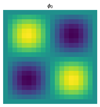
# condición inicial

Lx, Ly, Nx, Ny = 1., 1., 20, 20
dx, dy = Lx / Nx, Ly / Ny

x = np.linspace(0, Lx, Nx)
y = np.linspace(0, Ly, Ny)

p0 = np.zeros((Ny,Nx))
for i in range(Ny):
    for j in range(Nx):
        p0[i,j] = np.sin(2.*math.pi*x[j])*np.sin(2.*math.pi*y[i])

import matplotlib.pyplot as plt

fig = plt.figure(dpi=100)
ax = plt.subplot(1,1,1)
ax.imshow(p0)
ax.set_xlabel('x')
ax.set_ylabel('y')
ax.set_title('$\phi_0$')
ax.axis('off')
plt.show()

De la misma manera que con la ecuación de convección 1D, la versión 2D también tiene solución analítica

from matplotlib import animation, rc
rc('animation', html='html5')

def update(i):
    ax.clear()
    ax.imshow(ps[i])
    ax.set_xlabel('x')
    ax.set_ylabel('y')
    ax.set_title(f't = {ts[i]:.3f}')
    ax.axis('off')
    return ax

def compute_sol(Ny, Nx, u, v, t):
    p = np.zeros((Ny,Nx))
    for i in range(Ny):
        for j in range(Nx):
            p[i,j] = np.sin(2.*math.pi*(x[j] - u*t))*np.sin(2.*math.pi*(y[i] - v*t))
    return p

u, v = 1, 1
ts = np.linspace(0,1,50)
ps = []
for t in ts:
    p = compute_sol(Ny, Nx, u, v, t)
    ps.append(p)

fig = plt.figure(dpi=100)
ax = plt.subplot(1,1,1)
anim = animation.FuncAnimation(fig, update, frames=len(ps), interval=200)
plt.close()

anim

Vamos a resolver la ecuación usando la siguiente red neuronal.

import torch
import torch.nn as nn

# PRO TIP: usar `sin` como función de activación :)

class Sine(nn.Module):
    def __init__(self):
        super().__init__()
    def forward(self, x):
        return torch.sin(x)

mlp = nn.Sequential(
    nn.Linear(3, 100),
    Sine(),
    nn.Linear(100, 100),
    Sine(),
    nn.Linear(100, 1)
)

from fastprogress.fastprogress import master_bar, progress_bar

N_STEPS = 10000
N_SAMPLES = 200
N_SAMPLES_0 = 100

optimizer = torch.optim.Adam(mlp.parameters())
criterion = torch.nn.MSELoss()
mlp.train()
u, v = 1., 1.

mb = progress_bar(range(1, N_STEPS+1))

for step in mb:

    # optimize for PDE
    X = torch.rand((N_SAMPLES, 3), requires_grad=True) # N, (X, Y, T)
    y_hat = mlp(X) # N, P
    grads, = torch.autograd.grad(y_hat, X, grad_outputs=y_hat.data.new(y_hat.shape).fill_(1), create_graph=True, only_inputs=True)
    dpdx, dpdy, dpdt = grads[:,0], grads[:,1], grads[:,2]
    pde_loss = criterion(dpdt, - u*dpdx - v*dpdy)

    # optimize for initial condition
    x = torch.rand(N_SAMPLES_0)
    y = torch.rand(N_SAMPLES_0)
    p0 = torch.sin(2.*math.pi*x / Lx)*torch.sin(2.*math.pi*y / Ly)

    X = torch.stack([  # N0, (X, Y, T = 0)
        x, y,
        torch.zeros(N_SAMPLES_0)
    ], axis=-1)
    y_hat = mlp(X) # N, P0
    ini_loss = criterion(y_hat, p0.unsqueeze(1))

    # optimize for boundary conditions
    t = torch.rand(N_SAMPLES_0)
    X0 = torch.stack([
        torch.zeros(N_SAMPLES_0),
        y,
        t
    ], axis=-1)
    y_0 = mlp(X0)

    X1 = torch.stack([
        torch.ones(N_SAMPLES_0),
        y,
        t
    ], axis=-1)
    y_1 = mlp(X1)
    bound_loss1 = criterion(y_0, y_1)
    Y0 = torch.stack([
        x,
        torch.zeros(N_SAMPLES_0),
        t
    ], axis=-1)
    y_0 = mlp(X0)

    Y1 = torch.stack([
        x,
        torch.ones(N_SAMPLES_0),
        t
    ], axis=-1)
    y_1 = mlp(X1)
    bound_loss2 = criterion(y_0, y_1)
    bound_loss = bound_loss1 + bound_loss2

    # update
    optimizer.zero_grad()
    loss = pde_loss + ini_loss + bound_loss
    loss.backward()
    optimizer.step()

    mb.comment = f'pde_loss {pde_loss.item():.5f} ini_loss {ini_loss.item():.5f} bound_loss {bound_loss.item():.5f}'

def run_mlp(Nx, Ny, dt, u, v):
    ps, pa, ts = [], [], []
    t = 0
    L = 1.
    dx, dy = L / Nx, L / Ny
    x, y = [], []
    for i in range(Ny+1):
        for j in range(Nx+1):
            x.append(j*dx)
            y.append(i*dy)
    x = torch.tensor(x)
    y = torch.tensor(y)
    mlp.eval()
    while t < 1.:
        with torch.no_grad():
            X = torch.stack([  # N, (X, Y, T)
                x, y,
                torch.ones(len(x))*t,
            ], axis=-1)
            p = mlp(X)
        ps.append(p.reshape(Ny+1,Nx+1))
        pa.append(compute_sol(Ny, Nx, u, v, t))
        ts.append(t)
        t += dt
    return ps, pa, ts

ps, pa, ts = run_mlp(33, 33, 0.01, u, v)

fig = plt.figure(dpi=100)
ax = plt.subplot(1,1,1)
anim = animation.FuncAnimation(fig, update, frames=len(ps), interval=200)
plt.close()

anim