Smith-Hutton Problem

En este post vamos a resolver el problema conocido como Smith-Hutton, en el que resolveremos la ecuación de convección 2D que ya conocemos del post anterior (en este caso nos interesa la solución estática final, sin evolución temporal).

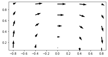
Se trata de un dominio rectangular en el cual tenemos una entrada por la parte inferior izquierda y una salida por la parte inferior derecha. El campo inicial de estará a cero, por lo que el valor indicado a la entrada viajará hasta la salida debido al campo de velocidad circular definido. Ya que no hay viscosidad, deberíamos encontrar a la salida exactamente el mismo perfil que a la entrada. Este problem es muy útil para evaluar diferentes esquemas numéricos y sus propiedades.

import numpy as np
import math

# condición inicial

Lx, Ly, Nx, Ny = 2., 1., 5, 5
dx, dy = Lx / Nx, Ly / Ny

x = np.linspace(-1+0.5*dx,1-0.5*dx,Nx)
y = np.linspace(0.5*dy,1-0.5*dy,Ny)
xx, yy = np.meshgrid(x, y)

p0 = np.zeros(Nx*Ny)

def velocity(x, y):
    return 2.*y*(1.-x**2.), -2.*x*(1.-y**2.)

import matplotlib.pyplot as plt

u, v = velocity(xx, yy)

fig, ax = plt.subplots()
ax.quiver(xx,yy,u,v)
ax.set_aspect('equal')
plt.show()

import torch
import torch.nn as nn

class Sine(nn.Module):
    def __init__(self):
        super().__init__()
    def forward(self, x):
        return torch.sin(x)

mlp = nn.Sequential(
    nn.Linear(2, 100),
    Sine(),
    nn.Linear(100, 100),
    Sine(),
    nn.Linear(100, 100),
    Sine(),
    nn.Linear(100, 100),
    Sine(),
    nn.Linear(100, 1)
)

from fastprogress.fastprogress import master_bar, progress_bar
import math

N_STEPS = 10000
N_SAMPLES = 200
N_SAMPLES_0 = 100

optimizer = torch.optim.Adam(mlp.parameters())
criterion = torch.nn.MSELoss()
mlp.train()
a = 10

mb = progress_bar(range(1, N_STEPS+1))

for step in mb:

    # optimize for PDE
    x = torch.rand(N_SAMPLES)*2. - 1.
    y = torch.rand(N_SAMPLES)
    X = torch.stack([
        x,
        y,
    ], axis=-1)
    X.requires_grad = True
    y_hat = mlp(X) # N, P
    grads, = torch.autograd.grad(y_hat, X, grad_outputs=y_hat.data.new(y_hat.shape).fill_(1), create_graph=True, only_inputs=True)
    dpdx, dpdy = grads[:,0], grads[:,1]
    u, v = velocity(X[:,0], X[:,1])
    pde_loss = criterion(u*dpdx, - v*dpdy)

    # optimize for boundary conditions
    # left
    y = torch.rand(N_SAMPLES_0)
    Y0 = torch.stack([
        torch.zeros(N_SAMPLES_0) - 1.,
        y,
    ], axis=-1)
    p_y0 = 1. - torch.ones(len(Y0))*math.tanh(a)
    y_y0 = mlp(Y0)
    y0_loss = criterion(y_y0, p_y0.unsqueeze(1))
    # right
    Y1 = torch.stack([
        torch.ones(N_SAMPLES_0),
        y,
    ], axis=-1)
    p_y1 = 1. - torch.ones(len(Y1))*math.tanh(a)
    y_y1 = mlp(Y1)
    y1_loss = criterion(y_y1, p_y1.unsqueeze(1))
    # top
    x = torch.rand(N_SAMPLES_0)*2. - 1.
    X1 = torch.stack([
        x,
        torch.ones(N_SAMPLES_0),
    ], axis=-1)
    p_x1 = 1. - torch.ones(len(X1))*math.tanh(a)
    y_x1 = mlp(X1)
    x1_loss = criterion(y_x1, p_x1.unsqueeze(1))
    # bottom (left)
    x = torch.rand(N_SAMPLES_0) - 1.
    X00 = torch.stack([
        x,
        torch.zeros(N_SAMPLES_0),
    ], axis=-1)
    p_x00 = 1. + torch.tanh(a*(2.*x + 1.))
    y_x00 = mlp(X00)
    x00_loss = criterion(y_x00, p_x00.unsqueeze(1))
    # bottom (right)
    x = torch.rand(N_SAMPLES_0)
    X01 = torch.stack([
        x,
        torch.zeros(N_SAMPLES_0),
    ], axis=-1)
    X01.requires_grad = True
    y_x01 = mlp(X01)
    grads, = torch.autograd.grad(y_x01, X01, grad_outputs=y_x01.data.new(y_x01.shape).fill_(1), create_graph=True, only_inputs=True)
    dpdy = grads[:,1]
    x01_loss = criterion(dpdy, torch.zeros(len(dpdy), 1))

    bound_loss = x00_loss + y0_loss + y1_loss + x1_loss + x01_loss

    # update
    optimizer.zero_grad()
    loss = pde_loss + bound_loss
    loss.backward()
    optimizer.step()

    mb.comment = f'pde_loss {pde_loss.item():.5f} bound_loss {bound_loss.item():.5f}'

C:\Users\sensio\miniconda3\lib\site-packages\torch\nn\modules\loss.py:520: UserWarning: Using a target size (torch.Size([100, 1])) that is different to the input size (torch.Size([100])). This will likely lead to incorrect results due to broadcasting. Please ensure they have the same size.
  return F.mse_loss(input, target, reduction=self.reduction)

def run_mlp(Nx, Ny):
    x = np.linspace(-1,1,Nx)
    y = np.linspace(0,1,Ny)
    X = np.stack(np.meshgrid(x,y), -1).reshape(-1, 2)
    X = torch.from_numpy(X).float()
    mlp.eval()
    with torch.no_grad():
        p = mlp(X)
    return p, x

Nx, Ny = 100, 50
p, x = run_mlp(Nx, Ny)

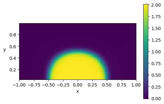
plt.figure(dpi=100)
plt.imshow(p.reshape(Ny,Nx), vmin=p.min(), vmax=p.max(), origin='lower',
           extent=[x.min(), x.max(), y.min(), y.max()])
plt.xlabel('x')
plt.ylabel('y    ', rotation=math.pi)
plt.colorbar()
plt.show()

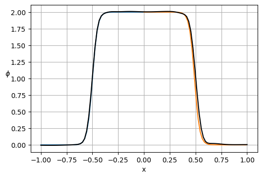
plt.figure(dpi=100)

x0 = x[x <= 0]
gt = 1. + np.tanh(a*(2*x0+1))

plt.plot(x0, gt)
plt.plot(x0 + 1., np.flip(gt))
plt.plot(x, p[:Nx], 'k')

plt.xlabel('x')
plt.ylabel('$\phi    $', rotation=math.pi)
plt.grid(True)
plt.show()

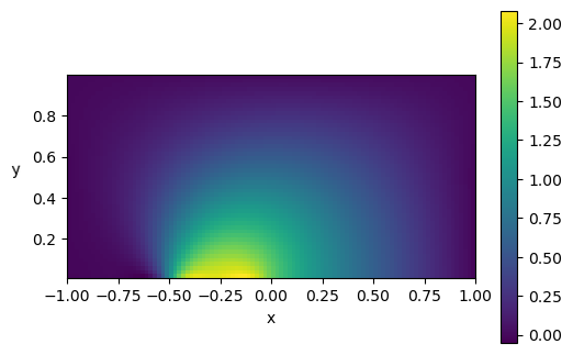
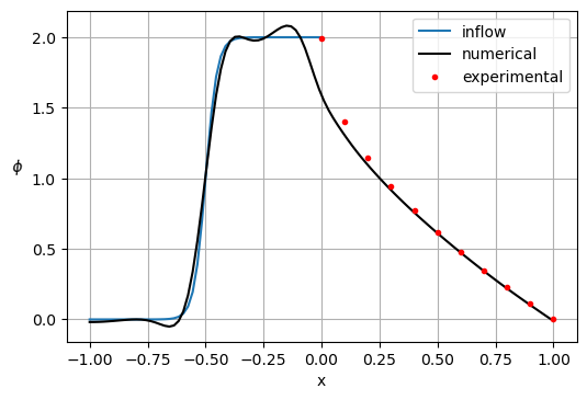
Añadiendo viscosidad

Otro benchmark interesante para evaluar métodos numéricos en la resolución de ecuaciones diferenciales consiste en resolver el mismo problema pero añadiendo viscosidad. La constante controlará cuánta viscosidad queremos en el problema. Además, ahora tenemos derivadas segundas. Gracias a Pytorch, calcular estas derivadas es muy sencillo.

mlp = nn.Sequential(
    nn.Linear(2, 100),
    Sine(),
    nn.Linear(100, 100),
    Sine(),
    nn.Linear(100, 100),
    Sine(),
    nn.Linear(100, 100),
    Sine(),
    nn.Linear(100, 1)
)

N_STEPS = 10000
N_SAMPLES = 200
N_SAMPLES_0 = 100

optimizer = torch.optim.Adam(mlp.parameters())
criterion = torch.nn.MSELoss()
mlp.train()
a = 10
g = 0.1

mb = progress_bar(range(1, N_STEPS+1))

for step in mb:

    # optimize for PDE
    x = torch.rand(N_SAMPLES)*2. - 1.
    y = torch.rand(N_SAMPLES)
    X = torch.stack([
        x,
        y,
    ], axis=-1)
    X.requires_grad = True
    y_hat = mlp(X) # N, P
    grads, = torch.autograd.grad(y_hat, X, grad_outputs=y_hat.data.new(y_hat.shape).fill_(1), create_graph=True, only_inputs=True)
    dpdx, dpdy = grads[:,0], grads[:,1]
    u, v = velocity(X[:,0], X[:,1])
    grads2, = torch.autograd.grad(dpdx, X, grad_outputs=dpdx.data.new(dpdx.shape).fill_(1), create_graph=True, only_inputs=True)
    dp2dx2 = grads2[:,0]
    grads2, = torch.autograd.grad(dpdy, X, grad_outputs=dpdy.data.new(dpdy.shape).fill_(1), create_graph=True, only_inputs=True)
    dp2dy2 = grads2[:,1]
    pde_loss = criterion(u*dpdx + v*dpdy, g*(dp2dx2 + dp2dy2))

    # optimize for boundary conditions
    # left
    y = torch.rand(N_SAMPLES_0)
    Y0 = torch.stack([
        torch.zeros(N_SAMPLES_0) - 1.,
        y,
    ], axis=-1)
    p_y0 = 1. - torch.ones(len(Y0))*math.tanh(a)
    y_y0 = mlp(Y0)
    y0_loss = criterion(y_y0, p_y0.unsqueeze(1))
    # right
    Y1 = torch.stack([
        torch.ones(N_SAMPLES_0),
        y,
    ], axis=-1)
    p_y1 = 1. - torch.ones(len(Y1))*math.tanh(a)
    y_y1 = mlp(Y1)
    y1_loss = criterion(y_y1, p_y1.unsqueeze(1))
    # top
    x = torch.rand(N_SAMPLES_0)*2. - 1.
    X1 = torch.stack([
        x,
        torch.ones(N_SAMPLES_0),
    ], axis=-1)
    p_x1 = 1. - torch.ones(len(X1))*math.tanh(a)
    y_x1 = mlp(X1)
    x1_loss = criterion(y_x1, p_x1.unsqueeze(1))
    # bottom (left)
    x = torch.rand(N_SAMPLES_0) - 1.
    X00 = torch.stack([
        x,
        torch.zeros(N_SAMPLES_0),
    ], axis=-1)
    p_x00 = 1. + torch.tanh(a*(2.*x + 1.))
    y_x00 = mlp(X00)
    x00_loss = criterion(y_x00, p_x00.unsqueeze(1))
    # bottom (right)
    x = torch.rand(N_SAMPLES_0)
    X01 = torch.stack([
        x,
        torch.zeros(N_SAMPLES_0),
    ], axis=-1)
    X01.requires_grad = True
    y_x01 = mlp(X01)
    grads, = torch.autograd.grad(y_x01, X01, grad_outputs=y_x01.data.new(y_x01.shape).fill_(1), create_graph=True, only_inputs=True)
    dpdy = grads[:,1]
    x01_loss = criterion(dpdy, torch.zeros(len(dpdy), 1))

    bound_loss = x00_loss + y0_loss + y1_loss + x1_loss + x01_loss

    # update
    optimizer.zero_grad()
    loss = pde_loss + bound_loss
    loss.backward()
    optimizer.step()

    mb.comment = f'pde_loss {pde_loss.item():.5f} bound_loss {bound_loss.item():.5f}'

C:\Users\sensio\miniconda3\lib\site-packages\torch\nn\modules\loss.py:520: UserWarning: Using a target size (torch.Size([100, 1])) that is different to the input size (torch.Size([100])). This will likely lead to incorrect results due to broadcasting. Please ensure they have the same size.
  return F.mse_loss(input, target, reduction=self.reduction)

Nx, Ny = 100, 50
p, x = run_mlp(Nx, Ny)

plt.figure(dpi=100)
plt.imshow(p.reshape(Ny,Nx), vmin=p.min(), vmax=p.max(), origin='lower',
           extent=[x.min(), x.max(), y.min(), y.max()])
plt.xlabel('x')
plt.ylabel('y    ', rotation=math.pi)
plt.colorbar()
plt.show()

# experimental results

exp = {
    'x': [0.0, 0.1, 0.2, 0.3, 0.4, 0.5, 0.6, 0.7, 0.8, 0.9, 1.0],
    'g_0.1': [1.989,1.402,1.146,0.946,0.775,0.621,0.480,0.349,0.227,0.111,0.0],
    'g_0.001': [2.0000,1.9990,1.9997,1.985,1.841,0.951,0.154,0.001,0.0,0.0,0.0],
    'g_0.000001': [2.0000,2.0,2.0,1.999,1.964,1.0,0.036,0.001,0.0,0.0,0.0]
}

plt.figure(dpi=100)

x0 = x[x <= 0]
gt = 1. + np.tanh(a*(2*x0+1))

plt.plot(x0, gt)
plt.plot(x, p[:Nx], 'k')
plt.plot(exp['x'], exp['g_0.1'], '.r')

plt.xlabel('x')
plt.ylabel('$\phi$    ', rotation=math.pi)
plt.grid(True)
plt.legend(['inflow', 'numerical', 'experimental'])
plt.show()

El hecho de usar una Red Neuronal como solución del problema nos permitiría incluso añadir el factor de viscosidad como input resolviendo un gran rango de casos a la vez, acelerando el proceso de optimización.