octubre 3, 2020
~ 24 MIN
Segmentación
< Blog RSS![]()
Segmentación
Seguimos explorando diferentes aplicaciones de visión artificial. En posts anteriores hemos hablado de localización y detección de objetos. En este caso exploraremos la tarea de segmentación semántica, consistente en clasificar todos y cada uno de los píxeles en una imagen.
Si bien en la tarea de clasificación consiste en asignar una etiqueta a una imagen en particular, en la tarea de segmentación tendremos que asignar una etiqueta a cada pixel produciendo mapas de segmentación, imágenes con la misma resolución que la imagen utilizada a la entrada de nuestro modelo en la que cada pixel es sustituido por una etiqueta.
En las arquitecturas que hemos utilizado en el resto de tareas, las diferentes capas convolucionales van reduciendo el tamaño de los mapas de características (ya sea por la configuración de filtros utilizados o el uso de pooling). Para hacer clasificación conectamos la salida de la última capa convolucional a un MLP para generar las predicciones, mientras que para la detección utilizamos diferentes capas convolucionales a diferentes escalas para generar las cajas y clasificación. En el caso de la segmentación necesitamos de alguna manera recuperar las dimensiones originales de la imagen. Vamos a ver algunos ejemplos de arquitecturas que consiguen esto mismo.
Arquitecturas
La primera idea que podemos probar es utilizar una CNN que no reduzca las dimensiones de los diferentes mapas de características, utilizando la correcta configuración de filtros y sin usar pooling.

Este tipo de arquitectura, sin embargo, no será capaz de extraer características a diferentes escalas y además será computacionalmente muy costos. Podemos aliviar estos problemas utilizando una arquitectura encoder-decoder, en la que en una primera etapa una CNN extrae características a diferentes escalas y luego otra CNN recupera las dimensiones originales.

Para poder utilizar este tipo de arquitecturas necesitamos alguna forma de incrementar la dimensión de un mapa de características. De entre las diferentes opciones, una muy utilizada es el uso de convoluciones traspuestas, una capa muy parecida a la capa convolucional que "aprende" la mejor forma de aumentar un mapa de características aplicando filtros que aumentan la resolución.
import torch

input = torch.randn(64, 10, 20, 20)
# aumentamos la dimensión x2
conv_trans = torch.nn.ConvTranspose2d(
    in_channels=10,
    out_channels=20,
    kernel_size=2,
    stride=2)
output = conv_trans(input)
output.shape
torch.Size([64, 20, 40, 40])
Puedes aprender más sobre esta operación en la documentación de Pytorch. De esta manera podemos diseñar arquitecturas más eficientes capaces de extraer información relevante a varias escalas. Sin embargo, puede ser un poco complicado recuperar información en el decoder simplemente a partir de la salida del encoder. Para resolver este problema se desarrolló una de las arquitecturas más conocidas y utilizadas para la segmentación: la red UNet.

Esta arquitectura es muy similar a la anterior, con la diferencia de que en cada etapa del decoder no solo entra la salida de la capa anterior sino también la salida de la capa correspondiente del encoder. De esta manera la red es capaz de aprovechar mucho mejor la información a las diferentes escalas.
Vamos a ver cómo implementar esta arquitectura para hacer segmentación de MRIs.
El Dataset
Podemos descargar un conjunto de imágenes de MRIs con sus correspondientes máscaras de segmentación usando el siguiente enlace.
import wget

url = 'https://mymldatasets.s3.eu-de.cloud-object-storage.appdomain.cloud/MRIs.zip'
wget.download(url)
'MRIs (6).zip'
import zipfile
with zipfile.ZipFile('MRIs.zip', 'r') as zip_ref:
    zip_ref.extractall('.')
Nuestro objetivo será el de segmentar una MRI cerebral para detectar la materia gris y blanca. Determinar la cantidad de ambas así como su evolución en el tiempo para un mismo paciente es clave para la detección temprana y tratamiento de enfermedades como el alzheimer.
import os
from pathlib import Path

path = Path('./MRIs')
imgs = [path/'MRIs'/i for i in os.listdir(path/'MRIs')]
ixs = [i.split('_')[-1] for i in os.listdir(path/'MRIs')]
masks = [path/'Segmentations'/f'segm_{ix}' for ix in ixs]

len(imgs), len(masks)
(425, 425)
import matplotlib.pyplot as plt
import numpy as np

fig, (ax1, ax2, ax3) = plt.subplots(1, 3, figsize=(30,10))
img = np.load(imgs[0])
mask = np.load(masks[0])
ax1.imshow(img)
ax2.imshow(mask)
ax3.imshow(img)
ax3.imshow(mask, alpha=0.4)
plt.show()
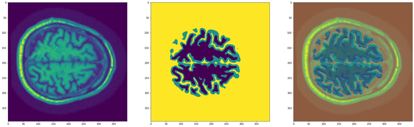
Nuestras imágenes tienen 394 x 394 píxeles, almacenadas como arrays de NumPy (que podemos cargar con la función np.load). Ya están normalizadas y en formato float32.
img.shape, img.dtype, img.max(), img.min()
((394, 394), dtype('float32'), 1.0093316, 0.00025629325)
En cuanto a las máscaras, también las tenemos guardadas como arrays de NumPy. En este caso el tipo es unit8, y la resolución es la misma que las de la imagen original. En cada píxel podemos encontrar tres posibles valores: 0, 1 ó 2. Este valor indica la clase (0 corresponde con materia blanca, 1 con materia gris, 2 con background).
mask.shape, mask.dtype, mask.max(), mask.min()
((394, 394), dtype('uint8'), 2, 0)
A la hora de entrenar nuestra red necesitaremos esta máscara en formato one-hot encoding, en el que extenderemos cada pixel en una lista de longitud igual al número de clases (en este caso 3) con valores de 0 en todas las posiciones excepto en aquella que corresponda con la clase, dónde pondremos un 1.
# one-hot encoding
mask_oh = (np.arange(3) == mask[...,None]).astype(np.float32)

mask_oh.shape, mask_oh.dtype, mask_oh.max(), mask_oh.min()
((394, 394, 3), dtype('float32'), 1.0, 0.0)
UNet
Vamos ahora a implementar nuestra red neuronal similar a UNet.
import torch.nn.functional as F

def conv3x3_bn(ci, co):
    return torch.nn.Sequential(
        torch.nn.Conv2d(ci, co, 3, padding=1),
        torch.nn.BatchNorm2d(co),
        torch.nn.ReLU(inplace=True)
    )

def encoder_conv(ci, co):
  return torch.nn.Sequential(
        torch.nn.MaxPool2d(2),
        conv3x3_bn(ci, co),
        conv3x3_bn(co, co),
    )

class deconv(torch.nn.Module):
    def __init__(self, ci, co):
        super(deconv, self).__init__()
        self.upsample = torch.nn.ConvTranspose2d(ci, co, 2, stride=2)
        self.conv1 = conv3x3_bn(ci, co)
        self.conv2 = conv3x3_bn(co, co)

    # recibe la salida de la capa anetrior y la salida de la etapa
    # correspondiente del encoder
    def forward(self, x1, x2):
        x1 = self.upsample(x1)
        diffX = x2.size()[2] - x1.size()[2]
        diffY = x2.size()[3] - x1.size()[3]
        x1 = F.pad(x1, (diffX, 0, diffY, 0))
        # concatenamos los tensores
        x = torch.cat([x2, x1], dim=1)
        x = self.conv1(x)
        x = self.conv2(x)
        return x

class UNet(torch.nn.Module):
    def __init__(self, n_classes=3, in_ch=1):
        super().__init__()

        # lista de capas en encoder-decoder con número de filtros
        c = [16, 32, 64, 128]

        # primera capa conv que recibe la imagen
        self.conv1 = torch.nn.Sequential(
          conv3x3_bn(in_ch, c[0]),
          conv3x3_bn(c[0], c[0]),
        )
        # capas del encoder
        self.conv2 = encoder_conv(c[0], c[1])
        self.conv3 = encoder_conv(c[1], c[2])
        self.conv4 = encoder_conv(c[2], c[3])

        # capas del decoder
        self.deconv1 = deconv(c[3],c[2])
        self.deconv2 = deconv(c[2],c[1])
        self.deconv3 = deconv(c[1],c[0])

        # útlima capa conv que nos da la máscara
        self.out = torch.nn.Conv2d(c[0], n_classes, 3, padding=1)

    def forward(self, x):
        # encoder
        x1 = self.conv1(x)
        x2 = self.conv2(x1)
        x3 = self.conv3(x2)
        x = self.conv4(x3)
        # decoder
        x = self.deconv1(x, x3)
        x = self.deconv2(x, x2)
        x = self.deconv3(x, x1)
        x = self.out(x)
        return x
model = UNet()
output = model(torch.randn((10,1,394,394)))
output.shape
torch.Size([10, 3, 394, 394])
Fit de 1 muestra
Para comprobar que todo funciona vamos a hacer el fit de una sola muestra. Para optimizar la red usamos la función de pérdida BCEWithLogitsLoss, que aplicará la función de activación sigmoid a las salidas de la red (para que estén entre 0 y 1) y luego calcula la función binary cross entropy.
device = "cuda" if torch.cuda.is_available() else "cpu"

def fit(model, X, y, epochs=1, lr=3e-4):
    optimizer = torch.optim.Adam(model.parameters(), lr=lr)
    criterion = torch.nn.BCEWithLogitsLoss()
    model.to(device)
    X, y = X.to(device), y.to(device)
    model.train()
    for epoch in range(1, epochs+1):
        optimizer.zero_grad()
        y_hat = model(X)
        loss = criterion(y_hat, y)
        loss.backward()
        optimizer.step()
        print(f"Epoch {epoch}/{epochs} loss {loss.item():.5f}")
img_tensor = torch.tensor(img).unsqueeze(0).unsqueeze(0)
mask_tensor = torch.tensor(mask_oh).permute(2, 0, 1).unsqueeze(0)

img_tensor.shape, mask_tensor.shape
(torch.Size([1, 1, 394, 394]), torch.Size([1, 3, 394, 394]))
fit(model, img_tensor, mask_tensor, epochs=20)
Epoch 1/20 loss 0.75874
Epoch 2/20 loss 0.73327
Epoch 3/20 loss 0.71612
Epoch 4/20 loss 0.70197
Epoch 5/20 loss 0.68919
Epoch 6/20 loss 0.67762
Epoch 7/20 loss 0.66688
Epoch 8/20 loss 0.65657
Epoch 9/20 loss 0.64672
Epoch 10/20 loss 0.63741
Epoch 11/20 loss 0.62850
Epoch 12/20 loss 0.61983
Epoch 13/20 loss 0.61144
Epoch 14/20 loss 0.60338
Epoch 15/20 loss 0.59573
Epoch 16/20 loss 0.58832
Epoch 17/20 loss 0.58104
Epoch 18/20 loss 0.57385
Epoch 19/20 loss 0.56678
Epoch 20/20 loss 0.55984
La función de pérdida va bajando, por lo que parece que está funcionando bien. Sin embargo, necesitamos alguna métrica para evaluar cuánto se parecen las máscaras predichas a las reales. Para ello podemos usar la métrica IoU, de la que ya hablamos anteriormente, y que calcula la relación entre la intersección y la unión de dos áreas.

def iou(outputs, labels):
    # aplicar sigmoid y convertir a binario
    outputs, labels = torch.sigmoid(outputs) > 0.5, labels > 0.5
    SMOOTH = 1e-6
    # BATCH x num_classes x H x W
    B, N, H, W = outputs.shape
    ious = []
    for i in range(N-1): # saltamos el background
        _out, _labs = outputs[:,i,:,:], labels[:,i,:,:]
        intersection = (_out & _labs).float().sum((1, 2))
        union = (_out | _labs).float().sum((1, 2))
        iou = (intersection + SMOOTH) / (union + SMOOTH)
        ious.append(iou.mean().item())
    return np.mean(ious)
def fit(model, X, y, epochs=1, lr=1e-3):
    optimizer = torch.optim.Adam(model.parameters(), lr=lr)
    criterion = torch.nn.BCEWithLogitsLoss()
    model.to(device)
    X, y = X.to(device), y.to(device)
    model.train()
    for epoch in range(1, epochs+1):
        optimizer.zero_grad()
        y_hat = model(X)
        loss = criterion(y_hat, y)
        loss.backward()
        optimizer.step()
        ious = iou(y_hat, y)
        print(f"Epoch {epoch}/{epochs} loss {loss.item():.5f} iou {ious:.5f}")
fit(model, img_tensor, mask_tensor, epochs=100)
Epoch 1/100 loss 0.55302 iou 0.25259
Epoch 2/100 loss 0.53576 iou 0.26911
Epoch 3/100 loss 0.50940 iou 0.31764
Epoch 4/100 loss 0.48882 iou 0.32311
Epoch 5/100 loss 0.46794 iou 0.32404
Epoch 6/100 loss 0.44806 iou 0.33351
Epoch 7/100 loss 0.42920 iou 0.33803
Epoch 8/100 loss 0.41053 iou 0.35249
Epoch 9/100 loss 0.39280 iou 0.35613
Epoch 10/100 loss 0.37601 iou 0.35847
Epoch 11/100 loss 0.36058 iou 0.35473
Epoch 12/100 loss 0.34442 iou 0.36439
Epoch 13/100 loss 0.32898 iou 0.36210
Epoch 14/100 loss 0.31499 iou 0.35568
Epoch 15/100 loss 0.30218 iou 0.35726
Epoch 16/100 loss 0.28931 iou 0.35301
Epoch 17/100 loss 0.27749 iou 0.35892
Epoch 18/100 loss 0.26667 iou 0.36389
Epoch 19/100 loss 0.25610 iou 0.35207
Epoch 20/100 loss 0.24597 iou 0.35379
Epoch 21/100 loss 0.23667 iou 0.35448
Epoch 22/100 loss 0.22762 iou 0.35760
Epoch 23/100 loss 0.21958 iou 0.34974
Epoch 24/100 loss 0.21201 iou 0.37263
Epoch 25/100 loss 0.20361 iou 0.35450
Epoch 26/100 loss 0.19585 iou 0.36176
Epoch 27/100 loss 0.18915 iou 0.37152
Epoch 28/100 loss 0.18330 iou 0.35609
Epoch 29/100 loss 0.17656 iou 0.37308
Epoch 30/100 loss 0.17063 iou 0.36349
Epoch 31/100 loss 0.16552 iou 0.37265
Epoch 32/100 loss 0.16094 iou 0.36155
Epoch 33/100 loss 0.15649 iou 0.39770
Epoch 34/100 loss 0.15201 iou 0.37829
Epoch 35/100 loss 0.14505 iou 0.39432
Epoch 36/100 loss 0.14219 iou 0.41538
Epoch 37/100 loss 0.13643 iou 0.40792
Epoch 38/100 loss 0.13326 iou 0.42131
Epoch 39/100 loss 0.12860 iou 0.46231
Epoch 40/100 loss 0.12504 iou 0.49150
Epoch 41/100 loss 0.12123 iou 0.51815
Epoch 42/100 loss 0.11726 iou 0.56154
Epoch 43/100 loss 0.11391 iou 0.62094
Epoch 44/100 loss 0.11008 iou 0.68132
Epoch 45/100 loss 0.10671 iou 0.72770
Epoch 46/100 loss 0.10315 iou 0.73970
Epoch 47/100 loss 0.09992 iou 0.75056
Epoch 48/100 loss 0.09664 iou 0.78678
Epoch 49/100 loss 0.09555 iou 0.79707
Epoch 50/100 loss 0.09354 iou 0.78773
Epoch 51/100 loss 0.08892 iou 0.82264
Epoch 52/100 loss 0.08626 iou 0.84145
Epoch 53/100 loss 0.08338 iou 0.83881
Epoch 54/100 loss 0.08002 iou 0.83426
Epoch 55/100 loss 0.07854 iou 0.84879
Epoch 56/100 loss 0.07535 iou 0.88240
Epoch 57/100 loss 0.07382 iou 0.87702
Epoch 58/100 loss 0.07140 iou 0.86407
Epoch 59/100 loss 0.06943 iou 0.87630
Epoch 60/100 loss 0.06758 iou 0.89681
Epoch 61/100 loss 0.06575 iou 0.89671
Epoch 62/100 loss 0.06408 iou 0.88863
Epoch 63/100 loss 0.06225 iou 0.90198
Epoch 64/100 loss 0.06066 iou 0.90992
Epoch 65/100 loss 0.05882 iou 0.91761
Epoch 66/100 loss 0.05741 iou 0.91286
Epoch 67/100 loss 0.05581 iou 0.92081
Epoch 68/100 loss 0.05439 iou 0.92696
Epoch 69/100 loss 0.05329 iou 0.92471
Epoch 70/100 loss 0.05202 iou 0.93076
Epoch 71/100 loss 0.05122 iou 0.92303
Epoch 72/100 loss 0.05119 iou 0.92157
Epoch 73/100 loss 0.05036 iou 0.90751
Epoch 74/100 loss 0.04850 iou 0.93188
Epoch 75/100 loss 0.04652 iou 0.93925
Epoch 76/100 loss 0.04632 iou 0.93021
Epoch 77/100 loss 0.04573 iou 0.93524
Epoch 78/100 loss 0.04415 iou 0.94054
Epoch 79/100 loss 0.04428 iou 0.92384
Epoch 80/100 loss 0.04344 iou 0.93099
Epoch 81/100 loss 0.04181 iou 0.93980
Epoch 82/100 loss 0.04121 iou 0.94207
Epoch 83/100 loss 0.03993 iou 0.95106
Epoch 84/100 loss 0.03943 iou 0.94642
Epoch 85/100 loss 0.03900 iou 0.94329
Epoch 86/100 loss 0.03762 iou 0.95671
Epoch 87/100 loss 0.03738 iou 0.95304
Epoch 88/100 loss 0.03661 iou 0.95044
Epoch 89/100 loss 0.03576 iou 0.95610
Epoch 90/100 loss 0.03546 iou 0.95723
Epoch 91/100 loss 0.03462 iou 0.95940
Epoch 92/100 loss 0.03410 iou 0.95693
Epoch 93/100 loss 0.03368 iou 0.96135
Epoch 94/100 loss 0.03306 iou 0.96258
Epoch 95/100 loss 0.03246 iou 0.96440
Epoch 96/100 loss 0.03206 iou 0.96363
Epoch 97/100 loss 0.03154 iou 0.96423
Epoch 98/100 loss 0.03107 iou 0.96700
Epoch 99/100 loss 0.03064 iou 0.96390
Epoch 100/100 loss 0.03020 iou 0.96516
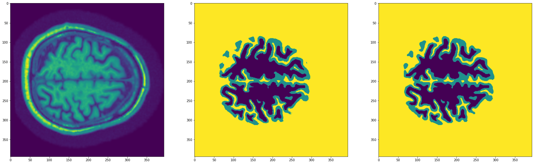
Ahora podemos generar predicciones para obtener máscaras de segmentación
model.eval()
with torch.no_grad():
    output = model(img_tensor.to(device))[0]
    pred_mask = torch.argmax(output, axis=0)

fig, (ax1, ax2, ax3) = plt.subplots(1, 3, figsize=(30,10))
ax1.imshow(img)
ax2.imshow(mask)
ax3.imshow(pred_mask.squeeze().cpu().numpy())
plt.show()
Entrenando con todo el dataset
Una vez hemos validado que nuestra red es capaz de hacer el fit de una imágen, podemos entrenar la red con todo el dataset.
class Dataset(torch.utils.data.Dataset):
  def __init__(self, X, y, n_classes=3):
    self.X = X
    self.y = y
    self.n_classes = n_classes

  def __len__(self):
    return len(self.X)

  def __getitem__(self, ix):
    img = np.load(self.X[ix])
    mask = np.load(self.y[ix])
    img = torch.tensor(img).unsqueeze(0)
    mask = (np.arange(self.n_classes) == mask[...,None]).astype(np.float32)
    return img, torch.from_numpy(mask).permute(2,0,1)
dataset = {
    'train': Dataset(imgs[:-100], masks[:-100]),
    'test': Dataset(imgs[-100:], masks[-100:])
}

len(dataset['train']), len(dataset['test'])
(325, 100)
dataloader = {
    'train': torch.utils.data.DataLoader(dataset['train'], batch_size=16, shuffle=True, pin_memory=True),
    'test': torch.utils.data.DataLoader(dataset['test'], batch_size=32, pin_memory=True)
}

imgs, masks = next(iter(dataloader['train']))
imgs.shape, masks.shape
(torch.Size([16, 1, 394, 394]), torch.Size([16, 3, 394, 394]))
from tqdm import tqdm

def fit(model, dataloader, epochs=100, lr=3e-4):
    optimizer = torch.optim.Adam(model.parameters(), lr=lr)
    criterion = torch.nn.BCEWithLogitsLoss()
    model.to(device)
    hist = {'loss': [], 'iou': [], 'test_loss': [], 'test_iou': []}
    for epoch in range(1, epochs+1):
      bar = tqdm(dataloader['train'])
      train_loss, train_iou = [], []
      model.train()
      for imgs, masks in bar:
        imgs, masks = imgs.to(device), masks.to(device)
        optimizer.zero_grad()
        y_hat = model(imgs)
        loss = criterion(y_hat, masks)
        loss.backward()
        optimizer.step()
        ious = iou(y_hat, masks)
        train_loss.append(loss.item())
        train_iou.append(ious)
        bar.set_description(f"loss {np.mean(train_loss):.5f} iou {np.mean(train_iou):.5f}")
      hist['loss'].append(np.mean(train_loss))
      hist['iou'].append(np.mean(train_iou))
      bar = tqdm(dataloader['test'])
      test_loss, test_iou = [], []
      model.eval()
      with torch.no_grad():
        for imgs, masks in bar:
          imgs, masks = imgs.to(device), masks.to(device)
          y_hat = model(imgs)
          loss = criterion(y_hat, masks)
          ious = iou(y_hat, masks)
          test_loss.append(loss.item())
          test_iou.append(ious)
          bar.set_description(f"test_loss {np.mean(test_loss):.5f} test_iou {np.mean(test_iou):.5f}")
      hist['test_loss'].append(np.mean(test_loss))
      hist['test_iou'].append(np.mean(test_iou))
      print(f"\nEpoch {epoch}/{epochs} loss {np.mean(train_loss):.5f} iou {np.mean(train_iou):.5f} test_loss {np.mean(test_loss):.5f} test_iou {np.mean(test_iou):.5f}")
    return hist
model = UNet()
hist = fit(model, dataloader, epochs=30)
loss 0.58465 iou 0.24777: 100%|██████████| 21/21 [00:07<00:00,  2.94it/s]
test_loss 0.66385 test_iou 0.08055: 100%|██████████| 4/4 [00:01<00:00,  3.88it/s]
  0%|          | 0/21 [00:00<?, ?it/s]


Epoch 1/30 loss 0.58465 iou 0.24777 test_loss 0.66385 test_iou 0.08055


loss 0.44370 iou 0.35166: 100%|██████████| 21/21 [00:07<00:00,  2.95it/s]
test_loss 0.44325 test_iou 0.22360: 100%|██████████| 4/4 [00:00<00:00,  4.08it/s]
  0%|          | 0/21 [00:00<?, ?it/s]


Epoch 2/30 loss 0.44370 iou 0.35166 test_loss 0.44325 test_iou 0.22360


loss 0.33856 iou 0.37663: 100%|██████████| 21/21 [00:07<00:00,  2.94it/s]
test_loss 0.31273 test_iou 0.35562: 100%|██████████| 4/4 [00:00<00:00,  4.10it/s]
  0%|          | 0/21 [00:00<?, ?it/s]


Epoch 3/30 loss 0.33856 iou 0.37663 test_loss 0.31273 test_iou 0.35562


loss 0.26632 iou 0.35184: 100%|██████████| 21/21 [00:07<00:00,  2.94it/s]
test_loss 0.25799 test_iou 0.31275: 100%|██████████| 4/4 [00:00<00:00,  4.05it/s]
  0%|          | 0/21 [00:00<?, ?it/s]


Epoch 4/30 loss 0.26632 iou 0.35184 test_loss 0.25799 test_iou 0.31275


loss 0.22021 iou 0.34264: 100%|██████████| 21/21 [00:07<00:00,  2.96it/s]
test_loss 0.21266 test_iou 0.34532: 100%|██████████| 4/4 [00:00<00:00,  4.07it/s]
  0%|          | 0/21 [00:00<?, ?it/s]


Epoch 5/30 loss 0.22021 iou 0.34264 test_loss 0.21266 test_iou 0.34532


loss 0.19001 iou 0.33456: 100%|██████████| 21/21 [00:07<00:00,  2.96it/s]
test_loss 0.18822 test_iou 0.32341: 100%|██████████| 4/4 [00:00<00:00,  4.10it/s]
  0%|          | 0/21 [00:00<?, ?it/s]


Epoch 6/30 loss 0.19001 iou 0.33456 test_loss 0.18822 test_iou 0.32341


loss 0.17054 iou 0.33296: 100%|██████████| 21/21 [00:07<00:00,  2.95it/s]
test_loss 0.17809 test_iou 0.36312: 100%|██████████| 4/4 [00:01<00:00,  3.82it/s]
  0%|          | 0/21 [00:00<?, ?it/s]


Epoch 7/30 loss 0.17054 iou 0.33296 test_loss 0.17809 test_iou 0.36312


loss 0.15606 iou 0.32807: 100%|██████████| 21/21 [00:07<00:00,  2.94it/s]
test_loss 0.16123 test_iou 0.33658: 100%|██████████| 4/4 [00:00<00:00,  4.07it/s]
  0%|          | 0/21 [00:00<?, ?it/s]


Epoch 8/30 loss 0.15606 iou 0.32807 test_loss 0.16123 test_iou 0.33658


loss 0.14524 iou 0.32532: 100%|██████████| 21/21 [00:07<00:00,  2.95it/s]
test_loss 0.15319 test_iou 0.35027: 100%|██████████| 4/4 [00:00<00:00,  4.09it/s]
  0%|          | 0/21 [00:00<?, ?it/s]


Epoch 9/30 loss 0.14524 iou 0.32532 test_loss 0.15319 test_iou 0.35027


loss 0.13672 iou 0.32426: 100%|██████████| 21/21 [00:07<00:00,  2.96it/s]
test_loss 0.13999 test_iou 0.31109: 100%|██████████| 4/4 [00:00<00:00,  4.10it/s]
  0%|          | 0/21 [00:00<?, ?it/s]


Epoch 10/30 loss 0.13672 iou 0.32426 test_loss 0.13999 test_iou 0.31109


loss 0.12915 iou 0.32757: 100%|██████████| 21/21 [00:07<00:00,  2.96it/s]
test_loss 0.13609 test_iou 0.34004: 100%|██████████| 4/4 [00:00<00:00,  4.11it/s]
  0%|          | 0/21 [00:00<?, ?it/s]


Epoch 11/30 loss 0.12915 iou 0.32757 test_loss 0.13609 test_iou 0.34004


loss 0.12244 iou 0.34689: 100%|██████████| 21/21 [00:07<00:00,  2.96it/s]
test_loss 0.13023 test_iou 0.38826: 100%|██████████| 4/4 [00:00<00:00,  4.06it/s]
  0%|          | 0/21 [00:00<?, ?it/s]


Epoch 12/30 loss 0.12244 iou 0.34689 test_loss 0.13023 test_iou 0.38826


loss 0.11529 iou 0.42372: 100%|██████████| 21/21 [00:07<00:00,  2.94it/s]
test_loss 0.11933 test_iou 0.45713: 100%|██████████| 4/4 [00:00<00:00,  4.05it/s]
  0%|          | 0/21 [00:00<?, ?it/s]


Epoch 13/30 loss 0.11529 iou 0.42372 test_loss 0.11933 test_iou 0.45713


loss 0.10654 iou 0.59694: 100%|██████████| 21/21 [00:07<00:00,  2.94it/s]
test_loss 0.11057 test_iou 0.61693: 100%|██████████| 4/4 [00:00<00:00,  4.10it/s]
  0%|          | 0/21 [00:00<?, ?it/s]


Epoch 14/30 loss 0.10654 iou 0.59694 test_loss 0.11057 test_iou 0.61693


loss 0.09833 iou 0.69466: 100%|██████████| 21/21 [00:07<00:00,  2.95it/s]
test_loss 0.10249 test_iou 0.69836: 100%|██████████| 4/4 [00:00<00:00,  4.06it/s]
  0%|          | 0/21 [00:00<?, ?it/s]


Epoch 15/30 loss 0.09833 iou 0.69466 test_loss 0.10249 test_iou 0.69836


loss 0.09082 iou 0.73460: 100%|██████████| 21/21 [00:07<00:00,  2.95it/s]
test_loss 0.09946 test_iou 0.71532: 100%|██████████| 4/4 [00:00<00:00,  4.11it/s]
  0%|          | 0/21 [00:00<?, ?it/s]


Epoch 16/30 loss 0.09082 iou 0.73460 test_loss 0.09946 test_iou 0.71532


loss 0.08657 iou 0.74121: 100%|██████████| 21/21 [00:07<00:00,  2.95it/s]
test_loss 0.09268 test_iou 0.71660: 100%|██████████| 4/4 [00:00<00:00,  4.09it/s]
  0%|          | 0/21 [00:00<?, ?it/s]


Epoch 17/30 loss 0.08657 iou 0.74121 test_loss 0.09268 test_iou 0.71660


loss 0.08128 iou 0.75008: 100%|██████████| 21/21 [00:07<00:00,  2.95it/s]
test_loss 0.09066 test_iou 0.72135: 100%|██████████| 4/4 [00:00<00:00,  4.07it/s]
  0%|          | 0/21 [00:00<?, ?it/s]


Epoch 18/30 loss 0.08128 iou 0.75008 test_loss 0.09066 test_iou 0.72135


loss 0.07691 iou 0.75876: 100%|██████████| 21/21 [00:07<00:00,  2.96it/s]
test_loss 0.08661 test_iou 0.72849: 100%|██████████| 4/4 [00:00<00:00,  4.10it/s]
  0%|          | 0/21 [00:00<?, ?it/s]


Epoch 19/30 loss 0.07691 iou 0.75876 test_loss 0.08661 test_iou 0.72849


loss 0.07308 iou 0.76545: 100%|██████████| 21/21 [00:07<00:00,  2.96it/s]
test_loss 0.08892 test_iou 0.71451: 100%|██████████| 4/4 [00:00<00:00,  4.07it/s]
  0%|          | 0/21 [00:00<?, ?it/s]


Epoch 20/30 loss 0.07308 iou 0.76545 test_loss 0.08892 test_iou 0.71451


loss 0.07026 iou 0.77062: 100%|██████████| 21/21 [00:07<00:00,  2.96it/s]
test_loss 0.07957 test_iou 0.74376: 100%|██████████| 4/4 [00:00<00:00,  4.04it/s]
  0%|          | 0/21 [00:00<?, ?it/s]


Epoch 21/30 loss 0.07026 iou 0.77062 test_loss 0.07957 test_iou 0.74376


loss 0.06722 iou 0.77535: 100%|██████████| 21/21 [00:07<00:00,  2.96it/s]
test_loss 0.07786 test_iou 0.74443: 100%|██████████| 4/4 [00:00<00:00,  4.08it/s]
  0%|          | 0/21 [00:00<?, ?it/s]


Epoch 22/30 loss 0.06722 iou 0.77535 test_loss 0.07786 test_iou 0.74443


loss 0.06689 iou 0.77016: 100%|██████████| 21/21 [00:07<00:00,  2.95it/s]
test_loss 0.08267 test_iou 0.70844: 100%|██████████| 4/4 [00:00<00:00,  4.04it/s]
  0%|          | 0/21 [00:00<?, ?it/s]


Epoch 23/30 loss 0.06689 iou 0.77016 test_loss 0.08267 test_iou 0.70844


loss 0.06428 iou 0.77814: 100%|██████████| 21/21 [00:07<00:00,  2.96it/s]
test_loss 0.08776 test_iou 0.69124: 100%|██████████| 4/4 [00:00<00:00,  4.10it/s]
  0%|          | 0/21 [00:00<?, ?it/s]


Epoch 24/30 loss 0.06428 iou 0.77814 test_loss 0.08776 test_iou 0.69124


loss 0.06285 iou 0.77859: 100%|██████████| 21/21 [00:07<00:00,  2.95it/s]
test_loss 0.07437 test_iou 0.74376: 100%|██████████| 4/4 [00:00<00:00,  4.08it/s]
  0%|          | 0/21 [00:00<?, ?it/s]


Epoch 25/30 loss 0.06285 iou 0.77859 test_loss 0.07437 test_iou 0.74376


loss 0.06006 iou 0.78755: 100%|██████████| 21/21 [00:07<00:00,  2.95it/s]
test_loss 0.07426 test_iou 0.74887: 100%|██████████| 4/4 [00:00<00:00,  4.14it/s]
  0%|          | 0/21 [00:00<?, ?it/s]


Epoch 26/30 loss 0.06006 iou 0.78755 test_loss 0.07426 test_iou 0.74887


loss 0.05860 iou 0.78809: 100%|██████████| 21/21 [00:07<00:00,  2.96it/s]
test_loss 0.08566 test_iou 0.68627: 100%|██████████| 4/4 [00:00<00:00,  4.03it/s]
  0%|          | 0/21 [00:00<?, ?it/s]


Epoch 27/30 loss 0.05860 iou 0.78809 test_loss 0.08566 test_iou 0.68627


loss 0.05978 iou 0.78113: 100%|██████████| 21/21 [00:07<00:00,  2.96it/s]
test_loss 0.08229 test_iou 0.72106: 100%|██████████| 4/4 [00:00<00:00,  4.07it/s]
  0%|          | 0/21 [00:00<?, ?it/s]


Epoch 28/30 loss 0.05978 iou 0.78113 test_loss 0.08229 test_iou 0.72106


loss 0.05583 iou 0.79455: 100%|██████████| 21/21 [00:07<00:00,  2.96it/s]
test_loss 0.07082 test_iou 0.74957: 100%|██████████| 4/4 [00:00<00:00,  4.06it/s]
  0%|          | 0/21 [00:00<?, ?it/s]


Epoch 29/30 loss 0.05583 iou 0.79455 test_loss 0.07082 test_iou 0.74957


loss 0.05405 iou 0.79965: 100%|██████████| 21/21 [00:07<00:00,  2.95it/s]
test_loss 0.06794 test_iou 0.75993: 100%|██████████| 4/4 [00:00<00:00,  4.11it/s]


Epoch 30/30 loss 0.05405 iou 0.79965 test_loss 0.06794 test_iou 0.75993
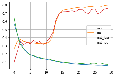
import pandas as pd
df = pd.DataFrame(hist)
df.plot(grid=True)
plt.show()
Transfer Learning
Podemos mejorar nuestros resultados si en vez de entrenar nuestra UNet desde cero utilizamos una red ya entrenada gracias al transfer learning. Para ello usaremos ResNet como backbone en el encoder de la siguiente manera.
import torchvision

class out_conv(torch.nn.Module):
    def __init__(self, ci, co, coo):
        super(out_conv, self).__init__()
        self.upsample = torch.nn.ConvTranspose2d(ci, co, 2, stride=2)
        self.conv = conv3x3_bn(ci, co)
        self.final = torch.nn.Conv2d(co, coo, 1)

    def forward(self, x1, x2):
        x1 = self.upsample(x1)
        diffX = x2.size()[2] - x1.size()[2]
        diffY = x2.size()[3] - x1.size()[3]
        x1 = F.pad(x1, (diffX, 0, diffY, 0))
        x = self.conv(x1)
        x = self.final(x)
        return x

class UNetResnet(torch.nn.Module):
    def __init__(self, n_classes=3, in_ch=1):
        super().__init__()

        self.encoder = torchvision.models.resnet18(pretrained=True)
        if in_ch != 3:
          self.encoder.conv1 = torch.nn.Conv2d(in_ch, 64, kernel_size=7, stride=2, padding=3, bias=False)

        self.deconv1 = deconv(512,256)
        self.deconv2 = deconv(256,128)
        self.deconv3 = deconv(128,64)
        self.out = out_conv(64, 64, n_classes)

    def forward(self, x):
        x_in = torch.tensor(x.clone())
        x = self.encoder.relu(self.encoder.bn1(self.encoder.conv1(x)))
        x1 = self.encoder.layer1(x)
        x2 = self.encoder.layer2(x1)
        x3 = self.encoder.layer3(x2)
        x = self.encoder.layer4(x3)
        x = self.deconv1(x, x3)
        x = self.deconv2(x, x2)
        x = self.deconv3(x, x1)
        x = self.out(x, x_in)
        return x
model = UNetResnet()
output = model(torch.randn((10,1,394,394)))
output.shape
torch.Size([10, 3, 394, 394])
model = UNetResnet()
hist = fit(model, dataloader, epochs=30)
  0%|          | 0/21 [00:00<?, ?it/s]
loss 0.47066 iou 0.45623: 100%|██████████| 21/21 [00:12<00:00,  1.64it/s]
test_loss 0.60641 test_iou 0.01456: 100%|██████████| 4/4 [00:01<00:00,  2.33it/s]
  0%|          | 0/21 [00:00<?, ?it/s]


Epoch 1/30 loss 0.47066 iou 0.45623 test_loss 0.60641 test_iou 0.01456


loss 0.35038 iou 0.67440: 100%|██████████| 21/21 [00:12<00:00,  1.64it/s]
test_loss 0.42464 test_iou 0.39127: 100%|██████████| 4/4 [00:01<00:00,  2.31it/s]
  0%|          | 0/21 [00:00<?, ?it/s]


Epoch 2/30 loss 0.35038 iou 0.67440 test_loss 0.42464 test_iou 0.39127


loss 0.30075 iou 0.71694: 100%|██████████| 21/21 [00:12<00:00,  1.64it/s]
test_loss 0.30222 test_iou 0.69314: 100%|██████████| 4/4 [00:01<00:00,  2.34it/s]
  0%|          | 0/21 [00:00<?, ?it/s]


Epoch 3/30 loss 0.30075 iou 0.71694 test_loss 0.30222 test_iou 0.69314


loss 0.26497 iou 0.73379: 100%|██████████| 21/21 [00:12<00:00,  1.65it/s]
test_loss 0.25938 test_iou 0.72612: 100%|██████████| 4/4 [00:01<00:00,  2.32it/s]
  0%|          | 0/21 [00:00<?, ?it/s]


Epoch 4/30 loss 0.26497 iou 0.73379 test_loss 0.25938 test_iou 0.72612


loss 0.23624 iou 0.74012: 100%|██████████| 21/21 [00:12<00:00,  1.64it/s]
test_loss 0.23491 test_iou 0.72937: 100%|██████████| 4/4 [00:01<00:00,  2.30it/s]
  0%|          | 0/21 [00:00<?, ?it/s]


Epoch 5/30 loss 0.23624 iou 0.74012 test_loss 0.23491 test_iou 0.72937


loss 0.20994 iou 0.75800: 100%|██████████| 21/21 [00:12<00:00,  1.64it/s]
test_loss 0.20987 test_iou 0.74493: 100%|██████████| 4/4 [00:01<00:00,  2.33it/s]
  0%|          | 0/21 [00:00<?, ?it/s]


Epoch 6/30 loss 0.20994 iou 0.75800 test_loss 0.20987 test_iou 0.74493


loss 0.18746 iou 0.77275: 100%|██████████| 21/21 [00:12<00:00,  1.64it/s]
test_loss 0.19024 test_iou 0.72724: 100%|██████████| 4/4 [00:01<00:00,  2.33it/s]
  0%|          | 0/21 [00:00<?, ?it/s]


Epoch 7/30 loss 0.18746 iou 0.77275 test_loss 0.19024 test_iou 0.72724


loss 0.16708 iou 0.79054: 100%|██████████| 21/21 [00:12<00:00,  1.64it/s]
test_loss 0.16811 test_iou 0.77223: 100%|██████████| 4/4 [00:01<00:00,  2.33it/s]
  0%|          | 0/21 [00:00<?, ?it/s]


Epoch 8/30 loss 0.16708 iou 0.79054 test_loss 0.16811 test_iou 0.77223


loss 0.15104 iou 0.79656: 100%|██████████| 21/21 [00:12<00:00,  1.64it/s]
test_loss 0.15827 test_iou 0.74552: 100%|██████████| 4/4 [00:01<00:00,  2.34it/s]
  0%|          | 0/21 [00:00<?, ?it/s]


Epoch 9/30 loss 0.15104 iou 0.79656 test_loss 0.15827 test_iou 0.74552


loss 0.13568 iou 0.81250: 100%|██████████| 21/21 [00:12<00:00,  1.64it/s]
test_loss 0.14146 test_iou 0.77153: 100%|██████████| 4/4 [00:01<00:00,  2.34it/s]
  0%|          | 0/21 [00:00<?, ?it/s]


Epoch 10/30 loss 0.13568 iou 0.81250 test_loss 0.14146 test_iou 0.77153


loss 0.12258 iou 0.82557: 100%|██████████| 21/21 [00:12<00:00,  1.64it/s]
test_loss 0.13118 test_iou 0.78280: 100%|██████████| 4/4 [00:01<00:00,  2.32it/s]
  0%|          | 0/21 [00:00<?, ?it/s]


Epoch 11/30 loss 0.12258 iou 0.82557 test_loss 0.13118 test_iou 0.78280


loss 0.11054 iou 0.84057: 100%|██████████| 21/21 [00:12<00:00,  1.64it/s]
test_loss 0.12378 test_iou 0.77133: 100%|██████████| 4/4 [00:01<00:00,  2.32it/s]
  0%|          | 0/21 [00:00<?, ?it/s]


Epoch 12/30 loss 0.11054 iou 0.84057 test_loss 0.12378 test_iou 0.77133


loss 0.10152 iou 0.84445: 100%|██████████| 21/21 [00:12<00:00,  1.64it/s]
test_loss 0.11357 test_iou 0.78920: 100%|██████████| 4/4 [00:01<00:00,  2.32it/s]
  0%|          | 0/21 [00:00<?, ?it/s]


Epoch 13/30 loss 0.10152 iou 0.84445 test_loss 0.11357 test_iou 0.78920


loss 0.09361 iou 0.85029: 100%|██████████| 21/21 [00:12<00:00,  1.64it/s]
test_loss 0.10501 test_iou 0.79471: 100%|██████████| 4/4 [00:01<00:00,  2.33it/s]
  0%|          | 0/21 [00:00<?, ?it/s]


Epoch 14/30 loss 0.09361 iou 0.85029 test_loss 0.10501 test_iou 0.79471


loss 0.08632 iou 0.85522: 100%|██████████| 21/21 [00:12<00:00,  1.64it/s]
test_loss 0.09837 test_iou 0.79835: 100%|██████████| 4/4 [00:01<00:00,  2.33it/s]
  0%|          | 0/21 [00:00<?, ?it/s]


Epoch 15/30 loss 0.08632 iou 0.85522 test_loss 0.09837 test_iou 0.79835


loss 0.07982 iou 0.86331: 100%|██████████| 21/21 [00:12<00:00,  1.64it/s]
test_loss 0.09293 test_iou 0.80176: 100%|██████████| 4/4 [00:01<00:00,  2.35it/s]
  0%|          | 0/21 [00:00<?, ?it/s]


Epoch 16/30 loss 0.07982 iou 0.86331 test_loss 0.09293 test_iou 0.80176


loss 0.07276 iou 0.87574: 100%|██████████| 21/21 [00:12<00:00,  1.64it/s]
test_loss 0.08955 test_iou 0.80167: 100%|██████████| 4/4 [00:01<00:00,  2.33it/s]
  0%|          | 0/21 [00:00<?, ?it/s]


Epoch 17/30 loss 0.07276 iou 0.87574 test_loss 0.08955 test_iou 0.80167


loss 0.06838 iou 0.87643: 100%|██████████| 21/21 [00:12<00:00,  1.64it/s]
test_loss 0.09200 test_iou 0.77620: 100%|██████████| 4/4 [00:01<00:00,  2.34it/s]
  0%|          | 0/21 [00:00<?, ?it/s]


Epoch 18/30 loss 0.06838 iou 0.87643 test_loss 0.09200 test_iou 0.77620


loss 0.06482 iou 0.87562: 100%|██████████| 21/21 [00:12<00:00,  1.65it/s]
test_loss 0.08966 test_iou 0.77144: 100%|██████████| 4/4 [00:01<00:00,  2.33it/s]
  0%|          | 0/21 [00:00<?, ?it/s]


Epoch 19/30 loss 0.06482 iou 0.87562 test_loss 0.08966 test_iou 0.77144


loss 0.06162 iou 0.87547: 100%|██████████| 21/21 [00:12<00:00,  1.64it/s]
test_loss 0.08233 test_iou 0.79512: 100%|██████████| 4/4 [00:01<00:00,  2.34it/s]
  0%|          | 0/21 [00:00<?, ?it/s]


Epoch 20/30 loss 0.06162 iou 0.87547 test_loss 0.08233 test_iou 0.79512


loss 0.05877 iou 0.87692: 100%|██████████| 21/21 [00:12<00:00,  1.64it/s]
test_loss 0.08195 test_iou 0.78903: 100%|██████████| 4/4 [00:01<00:00,  2.35it/s]
  0%|          | 0/21 [00:00<?, ?it/s]


Epoch 21/30 loss 0.05877 iou 0.87692 test_loss 0.08195 test_iou 0.78903


loss 0.05420 iou 0.88820: 100%|██████████| 21/21 [00:12<00:00,  1.65it/s]
test_loss 0.07881 test_iou 0.79599: 100%|██████████| 4/4 [00:01<00:00,  2.33it/s]
  0%|          | 0/21 [00:00<?, ?it/s]


Epoch 22/30 loss 0.05420 iou 0.88820 test_loss 0.07881 test_iou 0.79599


loss 0.05144 iou 0.88951: 100%|██████████| 21/21 [00:12<00:00,  1.65it/s]
test_loss 0.07565 test_iou 0.80191: 100%|██████████| 4/4 [00:01<00:00,  2.34it/s]
  0%|          | 0/21 [00:00<?, ?it/s]


Epoch 23/30 loss 0.05144 iou 0.88951 test_loss 0.07565 test_iou 0.80191


loss 0.04932 iou 0.88933: 100%|██████████| 21/21 [00:12<00:00,  1.65it/s]
test_loss 0.07559 test_iou 0.79975: 100%|██████████| 4/4 [00:01<00:00,  2.35it/s]
  0%|          | 0/21 [00:00<?, ?it/s]


Epoch 24/30 loss 0.04932 iou 0.88933 test_loss 0.07559 test_iou 0.79975


loss 0.04772 iou 0.88783: 100%|██████████| 21/21 [00:12<00:00,  1.65it/s]
test_loss 0.07180 test_iou 0.80552: 100%|██████████| 4/4 [00:01<00:00,  2.32it/s]
  0%|          | 0/21 [00:00<?, ?it/s]


Epoch 25/30 loss 0.04772 iou 0.88783 test_loss 0.07180 test_iou 0.80552


loss 0.04463 iou 0.89550: 100%|██████████| 21/21 [00:12<00:00,  1.64it/s]
test_loss 0.07281 test_iou 0.79339: 100%|██████████| 4/4 [00:01<00:00,  2.35it/s]
  0%|          | 0/21 [00:00<?, ?it/s]


Epoch 26/30 loss 0.04463 iou 0.89550 test_loss 0.07281 test_iou 0.79339


loss 0.04281 iou 0.89712: 100%|██████████| 21/21 [00:12<00:00,  1.65it/s]
test_loss 0.07053 test_iou 0.80255: 100%|██████████| 4/4 [00:01<00:00,  2.35it/s]
  0%|          | 0/21 [00:00<?, ?it/s]


Epoch 27/30 loss 0.04281 iou 0.89712 test_loss 0.07053 test_iou 0.80255


loss 0.03986 iou 0.90592: 100%|██████████| 21/21 [00:12<00:00,  1.64it/s]
test_loss 0.07449 test_iou 0.78764: 100%|██████████| 4/4 [00:01<00:00,  2.34it/s]
  0%|          | 0/21 [00:00<?, ?it/s]


Epoch 28/30 loss 0.03986 iou 0.90592 test_loss 0.07449 test_iou 0.78764


loss 0.03961 iou 0.89910: 100%|██████████| 21/21 [00:12<00:00,  1.64it/s]
test_loss 0.06947 test_iou 0.80261: 100%|██████████| 4/4 [00:01<00:00,  2.35it/s]
  0%|          | 0/21 [00:00<?, ?it/s]


Epoch 29/30 loss 0.03961 iou 0.89910 test_loss 0.06947 test_iou 0.80261


loss 0.03741 iou 0.90543: 100%|██████████| 21/21 [00:12<00:00,  1.64it/s]
test_loss 0.06850 test_iou 0.80490: 100%|██████████| 4/4 [00:01<00:00,  2.33it/s]


Epoch 30/30 loss 0.03741 iou 0.90543 test_loss 0.06850 test_iou 0.80490
import pandas as pd
df = pd.DataFrame(hist)
df.plot(grid=True)
plt.show()
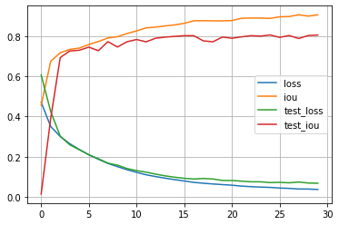
En este caso observamos como la red converge más rápido, sin embargo no obtenemos una gran mejora de prestaciones ya que nuestro dataset es muy pequeño y la naturaleza de las imágenes es muy distinta a las utilizadas para entrenar ResNet. Podemos generar máscaras para imágenes del dataset de test de la siguiente manera.
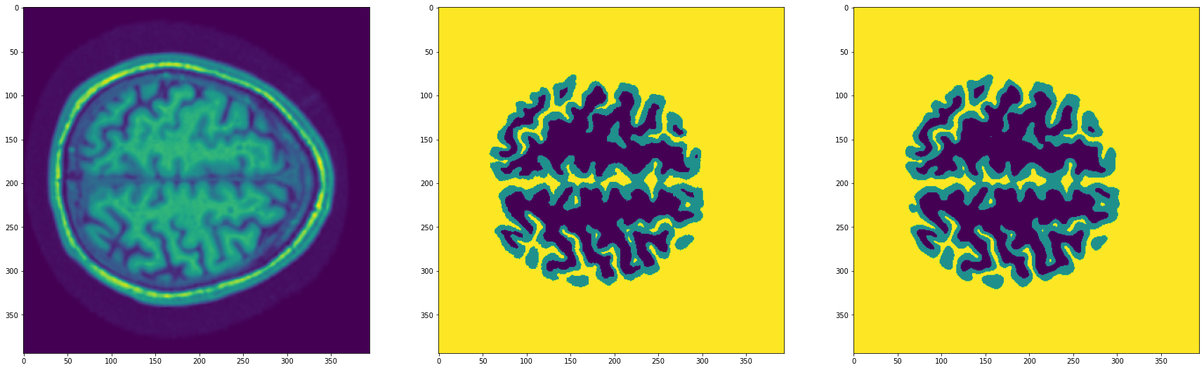
import random

model.eval()
with torch.no_grad():
    ix = random.randint(0, len(dataset['test'])-1)
    img, mask = dataset['test'][ix]
    output = model(img.unsqueeze(0).to(device))[0]
    pred_mask = torch.argmax(output, axis=0)

fig, (ax1, ax2, ax3) = plt.subplots(1, 3, figsize=(30,10))
ax1.imshow(img.squeeze(0))
ax2.imshow(torch.argmax(mask, axis=0))
ax3.imshow(pred_mask.squeeze().cpu().numpy())
plt.show()
Resumen
En este post hemos visto como podemos implementar y entrenar una red convolucional para llevar a cabo la tarea de segmentación semántica. Esta tarea consiste en clasificar todos y cada uno de los píxeles en una imagen. De esta manera podemos producir máscaras de segmentación que nos permiten localizar los diferentes objetos presentes en una imagen de forma mucho más precisa que la que podemos conseguir con la detección de objetos. Este tipo de tarea puede utilizarse en aplicaciones como la conducción autónoma o sistemas de diagnóstico médico, como hemos visto en el ejemplo de este post.